An Introduction to Linear Algebra
I hope that this little introduction to linear algebra helps you appreciate what it really is. I think the first time I saw linear algebra someone was like, “here’s a sysmtem of equations, let’s write it all these coefficients down in a box. Let’s call this box a matrix. yay now we can solve linear systems of equations by just manipulating this box. wooo.” I think this isn’t the best way to go about it. So, while representing linear transformations in terms of matrices is nice, and solving systems of equations is also nice, I am not going to write down any matrices today. I’m just going to talk to you about vector spaces and structure preserving maps between vector spaces (aka linear maps). I think that this angle will be a little bit different than other stuff out there, although maybe not. Anyways, I hope you enjoy it!
Vector Space
Well let’s get right to it, no messing around here:
Definition. Roughly speaking, A vector space is a set of objects called vectors along with a set of objects called scalars, where the notion of addition of vectors and multiplication of vectors by scalars makes sense. Furthermore addition and scaling of vectors play nicely, in particular playing nicely with scalars being added and multiplied.
Before I make this a bit more precise (e.g. defining nice) I think it’s better that I provide some examples of vector spaces to illustrate what is similar between them.
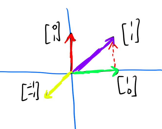
Example. The most classic of all examples: the set of vectors is \(\mathbb{R}^n\), and the set of scalars is \(\mathbb{R}\). \(\mathbb{R}^n\) refers to the set of \(n\)-element lists of real numbers. Consider \(\mathbb{R}^2\). Some vectors in \(\mathbb{R}^2\) are
- \((0, 1)\)
- \((1, 0)\)
- \((1, 1)\)
- \((0, -1)\)
- \((5, 6)\)
- \((-\pi, e)\)
We can add vectors via the rule: \((x_1,x_2)+(y_1, y_2) = (x_1+y_1, x_2+y_2)\). We can scale vectors via the rule: \(k(x_1,x_2) = (kx_1, kx_2)\).
This vector space very easily permits visualization, by placing the vectors in the plane.
Vector addition is accomplished gemoetrically by placing vectors “tip to tail” and going from the tip of start of the first vector to the end of the last vector.
Scalar multiplication is accomplished by shrinking/growing the vectors.
Some important properties to note about this vector space (these generalize):
Adding \((0,0)\) to vectors doesn’t change them: \((x,y)+(0,0) = (x,y)\). Multiplying vectors by \(0\) gives to \((0,0)\).
For every vector \((a,b)\), there is another vector, namely \((-a,-b)\), such that \((a,b)+(-a,-b) = (0,0)\).
Let \(x, y, z\) be vectors, let \(c, k\) be scalars. \[x+y = y+x.\]
\[(x+y)+z = x+(y+z).\]
\[c(k(x)) = (ck)x.\]
\[(c+k)x = cx + kx.\]
\[c(x+y) = cx + cy.\]
Another thing that is implicit in this all is the idea of “closure”. \(x+y\) needs to be a vector for any vectors \(x,y\), and also \(kx\) needs to be a vector for any vector \(x\) and any scalar \(k\).
Also, if you don’t know what a field is, don’t worry about it. A field is just a set with multiplication and addition that play really nicely with it. Usually this will be \(\mathbb{R}\) for us, although there are some other cool fields (e.g. finite fields, complex numbers).
Definition. Now we formally define a vector space. A vector space \(V\) over a field \(\mathbb{K}\) is a set of vectors \(V\) and scalars \(\mathbb{K}\) satisfying the following axioms:
Let \(0\in V\) denote the zero-vector (it’s properties are defined in the axioms below). Let \(x,y,z \in V\) let \(c,k \in \mathbb{K}\).
- “Additive axioms”:
- \(x+y=y+x\) (commutativity of addition)
- \((x+y)+z = x+(y+z)\) (associativity of addition)
- \(0+x = x+0 = x\)
- There is an inverse element \(-x\) such that \((-x) + x = 0\)
- “Multplicative axioms”:
- \(0x = 0\)
- \(1x = 1\)
- \((ck)x = c(k(x))\)
- “Distributive axioms”
- \(c(x+y) = cx + cy\)
- \((c+k)x = cx + kx\)
- “Closure axioms”
- \(x+y \in V\)
- \(cx \in V\)
OK. So probably none of these definitions were very surprising. I’ll give some more examples of vector spaces now, and then we’ll start talking about functions between vector spaces!
Example. The vector space (over the reals) of polynomials with real coefficients \(\mathbb{R}[x]\). Addition and multiplication is defined component-wise, i.e.
\[k \sum p_j x^j = \sum kp_j x^j \]
\[\sum a_j x^j + \sum b_j x^j = \sum (a_j + b_j) x^j.\]
You can say things like \[(3x^2 + x + 2) + 5x = 3x^2 + 6x + 2.\] And \[4(x+1) = 4x+4.\]
The \(0\)-polynomial satisfies the required conditions, additive inverses are achieved by negating polynomial’s coefficients i.e. \(x+1 + (-x-1) = 0\).
Example. Functions \(f: \mathbb{N}\to \mathbb{R}\) (vector space over the reals).
Addition is defined point-wise, i.e.
\(f + g\) is a function such that \((f+g)(x) = f(x) + g(x)\) for all \(x\in\mathbb{N}\). \(kf\) is a function with \((kf)(x) = kf(x)\).
Some examples are:
- \(f(x) = \sqrt{x}.\)
- \(f(x) = x\).
- \(f(x) = \sqrt{2} x.\)
- \(f(x) = x^2\).
- \(f(x) = 0.\)
- \(f(x) =\) the number of numbers less than \(x\) that are relatively prime to \(x\) (i.e.the number of \(y<x\) such that \(gcd(x,y) = 1\)).
Example. \(\mathbb{R}^\mathbb{N}\) (over the reals). This is the space of infinite sequences. Elements include vectors like
\[(1, 1/2, 1/3, 1/4, \ldots)\] and \[(0,0,0,\ldots).\]
Addition and multiplication is defined point-wise:
\[(a_1,\ldots) + (b_1, \ldots) = (a_1+b_1, \ldots)\] \[k(a_1,\ldots) = (ka_1, \ldots).\]
This vector space might be starting to look familiar. Could it be, this is “the same” vector space as the space of functions from the natural numbers to the real numbers? (yes!, more on this later)
OK I’ll do a couple more quick examples and then start talking about linear transformations. I’m getting there, I promise!
Example. \(\mathbb{C}\) over \(\mathbb{C}\). Enough said.
Example. The space of continuous functions on \([0,1]\).
Example. \((\mathbb{Z}/2\mathbb{Z})^n\) the space of binary strings of length \(n\).
I’ll just comment on addition in \(\mathbb{Z}/2\mathbb{Z}\) for a second.
\(1+1 = 0\), \(1+0= 1\), \(0+0 = 0.\) Sound crazy? It’s not. You could interpret \(1,0\) as true, false, and then this is NAND (i.e. NOT AND). You could also just think of it as addition mod 2.
Anyways, there are a lot of reasons why you might want the set of binary strings of length \(n\). High quality vector space right there.
OK, I’m far from being done, but it’s 1:01 (am). wow that rhymed. Anyways, I’m trying to get to bed earlier than normal today, so we’re gonna move on.
Linear Transformations
Definition. A linear transformation between vector spaces \(V, W\) is a function \(T: V\to W\) that plays nicely with vector addition and scaling. In particular \(T\) must satisfy:
\[T(x+y) = T(x) + T(y)\] and \[T(kx) = kT(x)\]
I would probably define linear algebra as “the study of vector spaces and linear maps between them”. but whatever.
Anyways, here’s some examples:
Example. Consider a map \(T : \mathbb{R}^2 \to \mathbb{R}^2\) that does \[(x, y) \mapsto (-y, x) \]
This map is linear. It does rotation by 90 degrees counter-clockwise.
Here is a visualization of this map acting on a set of points: 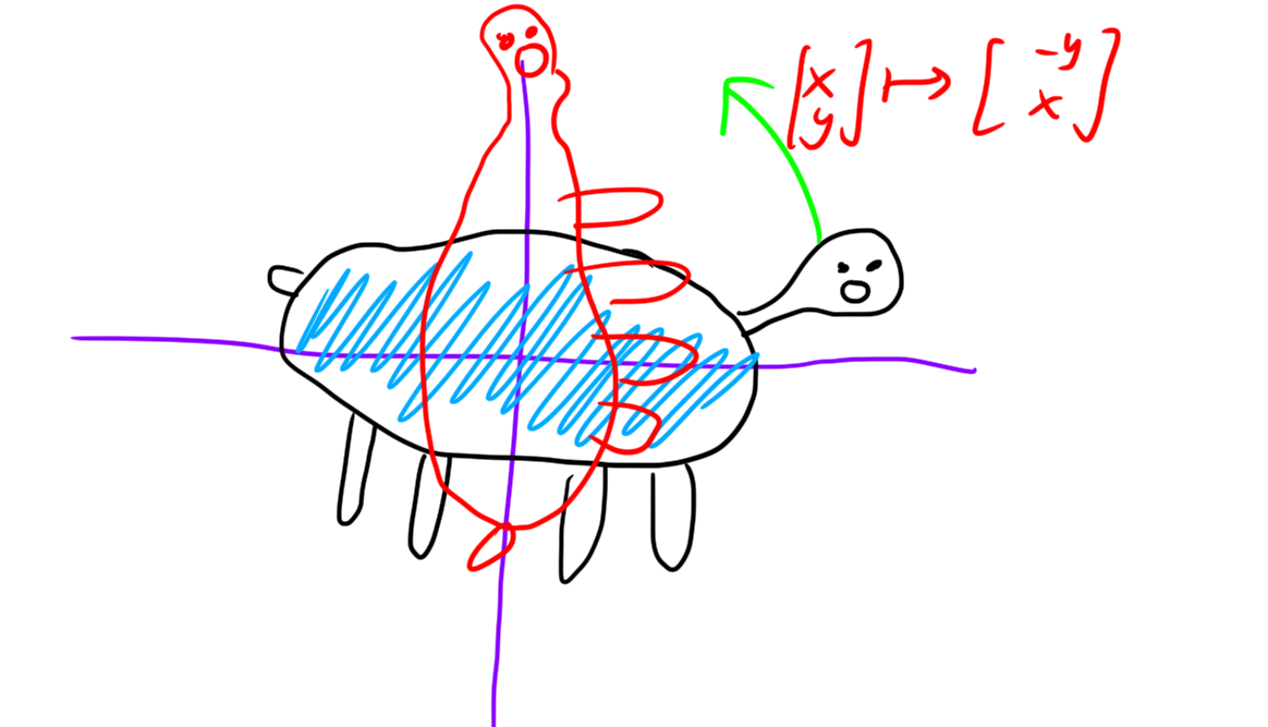
Example. Consider a map \(T : \mathbb{R}^2 \to \mathbb{R}^2\) that does \[(x, y) \mapsto (2x, 2y) \]
This map is linear. It scales vectors up.
Example. Consider a map \(T : \mathbb{R}^2 \to \mathbb{R}^2\) that does \[(x, y) \mapsto \left(\frac{3}{5} x + \frac{4}{5} y\right)(3/5, 4/5).\]
This map does projection onto the line \(y=\frac{4}{3}x.\)
Example. Let \(P_n\) be the space of polynomials of degree at most \(n\). The map \(T: P_n \to P_n\) \[T(p) = p'\] (the derivative) is linear.
Example. Let \(P_n\) be the space of polynomials of degree at most \(n\). The map \(T: P_n \to \mathbb{R}^3\) \[T(p) = (p(1), p(2), p(3))\] is linear.
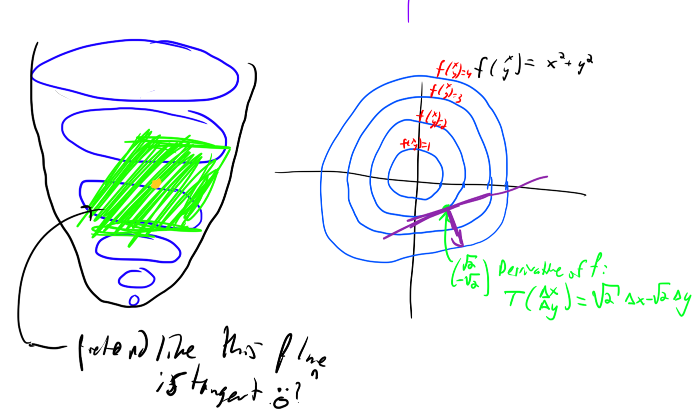
Remark. Sometimes we care about non-linear maps between vector spaces. But these are pretty hard to understand. So instead, it is really useful often to use linear approximations of non-linear maps to try to understand them.
The derivative of a function is defined to be the best linear approximation to it.
For example, the derivative of the function \(f(x,y) = x^2 + y^2\) at the point \((a,b)\) is the function \(T(\Delta x,\Delta y) = 2a\Delta x + 2b\Delta y.\) Note that \(T\) does not take in the actual values \(x,y\) but rather \(\Delta x\) and \(\Delta y\), which are defined as \(x-a, y-b\). And \(T\) outputs the difference from \(f(a,b)\). Thus the approxmiation to \(f\) is really \[f(x,y) \approx T(x-a, y-b) + f(a,b).\] However of course, this function is not linear in \(x,y\)! But \(T\) is linear in \(\Delta x, \Delta y\).
Note: if you were taught in some single-variable calculus course that the derivative of a function is a number abandon this notion right now!!!! The derivative is the best linear approximation to a function. In \(\mathbb{R}\) there happens to be an easy way to associate linear functions with numbers (the slope of the function). This doesn’t generalize. It’s way better to think of derrivatives as linear functions that do the best job at approximating the function.
Invertible linear maps are a very important type of linear map. For instance, they can be used to define what it means for two vector spaces to be “the same”:
Definition. Two vector spaces are said to be isomorphic, written \(V \cong W\) if there exists an invertible linear map \(\phi : V\to W\) (that is \(\phi\) must be onto \(W\) and must be one to one).
Example. The vector space of polynomials wtih real coefficients of degree \(2\) or less, denote \(P_2\), is isomprphic to \(\mathbb{R}^3\). In particular, we can associate the polynomial \(ax^2 + bx + c \in P_2\) with, for instance, \((a,b,c) \in\mathbb{R}^3.\) This map is clearly an isomorphism.
Bases
Given a set, an interesting question to ask is “how big is this set”. For almost all of the vector spaces we’ve discussed though, the set of vectors is infinite (in fact often uncountably infinite!) so this wouldn’t be a very satisfying thing. However, we can define a notion of largeness of a vector space, dimension based on the minimal number of vectors required to be able to reach all the vectors in a space. Now I’ll define this more formally.
Definition. A linear combination of a set of vectors \(\left\{ v_1,\ldots, v_n\right\}\) is a vector of the form \[\sum_{i=1}^n \alpha_i v_i\] for some scalars \(\alpha_i\).
Definition. A set of vectors \(\left\{ v_1, \ldots, v_n\right\}\) is said to span a vector space \(V\) if any vector \(v \in V\) can be expressed as some linear combination of \(v_1,\ldots, v_n\). i.e. there must exist \(\alpha_i\) such that \[v = \sum_{i} \alpha_i v_i.\]
Definition. We write the set of all linear combinations of \(v_1,\ldots, v_n\) as \[[v_1, \ldots, v_n]\] This is the span of \(v_1, \ldots, v_n\).
\(v_1, \ldots, v_n\) spans a vector space \(V\) if \(V \subset [v_1,\ldots,v_n]\).
However, we are interested in a minimal spanning set.
Definition. A minimal spanning set for a vector space \(V\) is a finite set of vectors \(v_i\) that spans the space, such that if you remove any vector \(v_i\) from the set, the resulting set of vectors no longer spans \(V\).
A minimal spanning set is also called a basis.
Remark. A basis for a vector space need not exist. If a vector space does not admit a basis then it is called an infinite dimensional vector space.
Example. The vector space of polynomials is infinite dimensional; it clearly admits no basis: imagine it did, then take a polynomial with degree more than the highest degree of the basis elements, this yields a contradiction.
Claim. We claim that the number of elements in a basis for \(V\) is unique.
Proof. Let \(V\) have two bases \(\left\{ v_1,\ldots, v_m\right\}\) and \(\left\{ w_1,\ldots, w_n\right\}\). We aim to show that \(m=n\).
As \(v_i\) spans \(V\) we can express each \(w_j\) as a linear combination of \(v_i\)’s. On the other hand, we can express each \(w_j\) as a linear combination of \(v_j\)’s.
Assume for contradiction that \(m \neq n\). Without loss of generality \(m < n\).
We inductively create a series of spanning sets:
- \(\left\{ v_1,\ldots, v_m\right\}\)
- \(\left\{ w_1, v_2, \ldots, v_m\right\}\) this is possible as the previous set was spanning, hence \(w_1\) can be written as a linear combination of \(v_i\)’s, and it must have a non-zero coefficient, which is on \(v_1\) without loss of generality
- \(\left\{ w_1, w_2, v_3, \ldots, v_m\right\}\) by the same logic
- \(\cdots\) (induction or whatever)
- \(\left\{ w_1,w_2,\ldots, w_m\right\}\)
But this can’t be spanning! It contradicts the minimality of the set \(\left\{ w_1,\ldots, w_n\right\}\), because we shouldn’t be able to remove \(w_{m+1},\ldots, w_n\) and still get a spanning set! Hence it is impossible for \(m \neq n\).
And thus the number of elements in a basis is well defined.
Definition. We call the dimension of a vector space the number of elements in a basis for it.
Example. The so called “standard basis” for \(\mathbb{R}^n\) is the set of vectors \(\left\{ (1,0,0,\ldots,0), (0,1,0,0,\ldots, 0), \ldots, (0,0,\ldots, 1)\right\}\) with the \(i\)-th standard basis vector \(e_i\) containing \(0\) in every component except a \(1\) in the \(i\)-th component.
Example. A basis for \(P_2\) is \(\left\{ 1, x, x^2\right\}\)
Example. An altenrative basis for \(\mathbb{R}^2\) is \(\left\{ (1,2), (2,1)\right\}\). Clearly this set spans the same space, but it is just a different way of representing points.
You can represent points like \((5,7)\) as \((5,7) = 3(1,2) + 1(2,1)\). Thus you could say that \((5,7)\)’s coordinates in the new basis rae \((3,1)\).
beign rmk There are situations in which change of basis can be incredibly helpful. For example, imagine that you are making a 3D game and you have a camera that you want to rotate to look at the player. There is a simple way to represent the camera’s rotation as a linear transformation relative the the camera’s local coordinates. But on the world coordinates this isn’t true. So you’d like to do a change of basis, to the new basis being a vector which is where the camera is looking at, a vector that is up for the camera, and a vector to the right. end rmk
Definition. A set \(v_1,\ldots, v_n\) of vectors is said to be linearly independent if no vector can be made as a linear combination of the other vectors. Equivalently, \[\sum_i \alpha_i v_i = 0 \,\,\,\, \implies \alpha_i = 0.\]
Claim. An equivalent definition of a basis is maximal linear independent set of vectors
Proof. left as an exercise to the reader
Image and Kernel
OK, now you’re ready to see a very cool result, the Rank Nullity Theorem. It is a relationship between two very important sets that give a lot of information about a linear transformation: the image and kernel of the linear transformation.
Definition. A subspace of a vector space \(V\) over \(\mathbb{K}\) is a subset \(M \subset V\) of the vectors that is closed under addition and multiplication.
That is, For any \(x,y\in M\) we have \(x+y \in M\), and for any \(c \in\mathbb{K}\) we have \(cx \in M\).
Example. A line through the origin in \(\mathbb{R}^2\) or \(\mathbb{R}^3\) is a subspace.
Example. Polynomials of degree at most \(2\) that have a zero at \(4\) are a subspace of the space of polynomials.
Remark. Note that any subspace contains the \(0\)-vector as this is necessary to be closed under multiplication.
Now, as promised, I define some really imporant subspaces.
Definition. The image of a linear transformation \(T : V\to W\) is the set \(\im(T) = \left\{ T(x)\; : \;x\in V \right\}.\) That is, the set of all vectors “hit” by \(T\); the set of all vectors \(y \in W\) so that there exists \(x \in V\) with \(T(x) = y\).
Definition. The kernel of a linear transformation \(T: V \to W\) is the set \(\ker(T) = \left\{ x \in V\; : \;T(x)= 0 \right\}.\) That is, the set of vectors sent to the zero vector.
I really like the following picture, showing graphically these spaces: 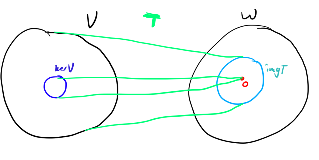
Theorem. Let \(T: V\to W\). \(\im(T)\) is a subspace of \(W\) and \(\ker(T)\) is a subspace of \(V\).
Proof. Take \(x,y \in \im(T)\subset W\), \(c\) a scalar. Then there must be \(a,b \in V\) with \(T(a) = x, T(b) = y\). Then \[T(a+cb) = T(a)+cT(b) = x+cy.\] So \(x+cy \in \im(T).\) Hence \(\im(T)\) is a subspace of \(W\), as it is closed under both scaling and addition.
Now take \(x, y\in \ker(T) \subset V\), \(c\) a scalar.
\[T(x+cy) = T(x) + cT(y) = 0+ c0 = 0+0 = 0.\] Hence \(\ker(T)\) is a subspace of \(V\), as it is closed under both scaling and addition.
Example. Consider the linear transformation \(T: \mathbb{R}^2 \to \mathbb{R}^3\), defined by \(T(x,y) = (x,0,0).\)
\(\im(T) = [(1,0,0)]\)
The Rank Nullity Theorem is a relationhsip between these subspaces, which I believe is “deep stuff”. I’ll state it now, but we’ll need one more idea before the proof.
Theorem. Let \(T: V \to W\) be a linear map. Then \[\dim\im(T) + \dim \ker T = \dim V.\]
Remark. \(\dim \im T\) is called the “rank” of \(T\), and \(\dim \ker T\) is called the “nullity” of \(T\).
Before proving this, we need a really cool idea: Quotient Spaces!!!
Definition. Let \(V\) be a vector space, and let \(M \subset V\) be a subspace of \(V\). Then the quotient space \(V/W\) (pronounced “\(V\) mod \(W\)”) is defined as \[V/W = \{W+x | x \in V\}.\]
Now we prove the following key fact:
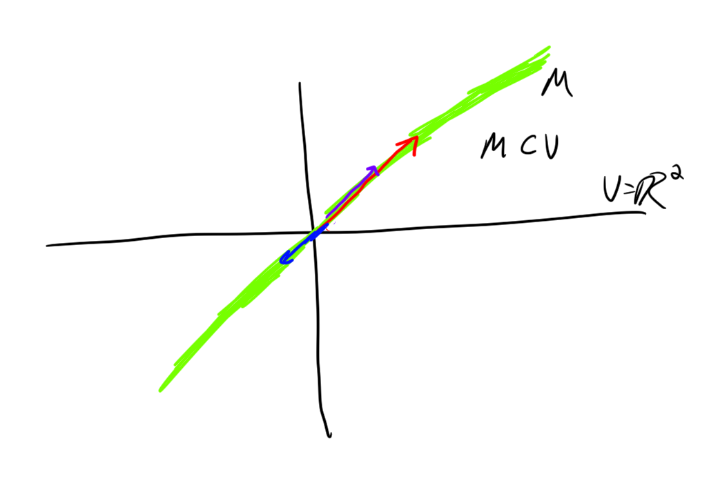
Theorem. (First Isomorphism Theorem)
Let \(T: V\to W\), then \[V/\ker T \cong \im T\]
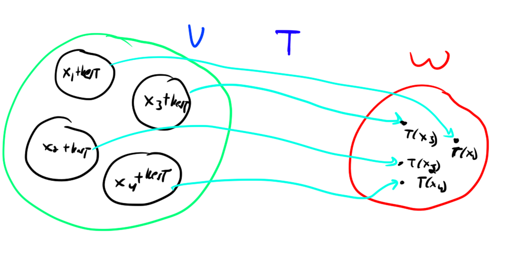
Proof. Consider \(x \in V/\ker T\). Let \(x = z+\ker T\) for arbitrary \(z\in x\). Note that for any \(y \in x\), \(T(y) = T(z).\) Hence it makes sense to say \(T(x) = T(z)\). We claim that \(\phi(z+\ker T) = T(z)\) is an isomorphism between \(V/\ker T\) and \(\im(T)\). First note that \(\phi\) is well defined because regardless of the chosen representative \(z \in x\), \(T(z)\) is the same.
To show that \(\phi\) is invertible we must show that it is one-to-one (doesn’t map different values to the same output) and also that it is onto (maps to each element of the codomain).
First we show \(\phi\) is one-to-one. If \(T(x) = T(y)\) then \(T(x-y) = 0\) so \(x-y \in \ker T\), as desired. Next, we show \(\phi\) is onto. Take any \(y \in \im(T)\). By definition there is some \(x \in V\) mapping to \(y\). Then all of the vectors in \(x+\ker T\) map to \(y\), as desired.
Hence the vector spaces are isomorphic.
Here’s a picture showing this:
Example. Consider the map \(T: P_2 \to P_2\) defined by \(ax^2 + bx + c\cdot 1 \mapsto ax+b\). \(\ker T = [1]\), \(\im T = [1, x]\). In \(P_2/\ker T\) we group together polynomials that differ by a constant, so \(P_2/\ker T = \left\{ \left\{ ax^2+bx+c\; : \;c\in \mathbb{R} \right\}\; : \;a,b\in\mathbb{R} \right\}.\) We can write this as \(P_2/\ker T = \left\{ ax^2+bx + \mathbb{R}\cdot 1\; : \;a,b\in\mathbb{R} \right\}.\) But this can easily be identified with \(\left\{ ax+b\; : \;a,b\in\mathbb{R} \right\}\). Hence \[P_2/\ker T \cong \im T.\]
Example. Consider the map \(T: \mathbb{R}^2 \to \mathbb{R}^2\) defined as \(T(x,y) = (x, y)\). \(\ker T = \left\{ 0\right\}\), and \(\mathbb{R}^2/\ker T = \left\{ \left\{ (x,y)\right\}\; : \;x,y\in \mathbb{R} \right\}\). But this is trivially identified with \(\mathbb{R}^2 = \im T\).
Example. Consider the map \(T: \mathbb{R}^3 \to \mathbb{R}^2\) defined as \(T(x,y,z) = (z, y)\). \(\ker T = [(1,0,0)]\), and \(\mathbb{R}^3/\ker T = \left\{ [(1,0,0)] + (0,y,z)\; : \;y, z\in \mathbb{R} \right\}\). But this is trivially identified with \(\mathbb{R}^2 = \im T\).
Example. Consider the map \(T: \mathbb{R}^3 \to \mathbb{R}^2\) defined as \(T(x,y,z) = (0, y)\). \(\ker T = [(1,0,0), (0,0,1)]\), and \(\mathbb{R}^3/\ker T = \left\{ [(1,0,0), (0,0,1)] + (0,y,0)\; : \;y\in \mathbb{R} \right\}\). But this is trivially identified with \([(0,1)] = \im T\).
I hope you get the point.
Now rank nullity is evident. We simply need a small Lemma on the dimension of Quotient spaces:
Lemma. Let \(V\) be a vector space, \(M \subset V\) be a subspace. \[\dim V/M = \dim V - \dim M.\]
Proof. Take a basis \(v_1,\ldots, v_m\) for \(M\), extend it to a basis \(v_1,\ldots, v_n\) for \(V\). Then \(M + v_{m+1}, \ldots, M+v_n\) is a basis for \(V/M\). The basis has \[n-m = \dim V - \dim M\] elements. Hence \[\dim V/M = \dim V - \dim M.\]
Proof. By the first isomorphism theorem \[V/\ker T = \im T.\] By our lemma this implies \[\dim V/\ker T = \dim V - \dim \ker T = \dim \im T\] as desired.
The End
If you’re interested in Linear Algebra totally learn more about it! It’s pretty awesome IMHO.