Vector Calculus
Rand: Hey, I really got nothing
Al: Just the area of a circle is 0 because a circle is a 1 dimensional submanifold of \(\mathbb{R}^2\)
Rand: Oh RW. What a guy.
Vector Calculus, Physics Edition
Note: we work in \(\mathbb{R}^3\) because physics. Or maybe actually \(\mathbb{R}^2\) so I can draw stuff.
A vector field is a function \(F: \mathbb{R}^3 \to \mathbb{R}^3\). Intuitively this can be thought of as associating to each point in space a vector. Vector fields can model fluid forces, wind, electric fields, and more abstractly things like population dynamics and stuff.
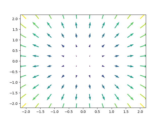
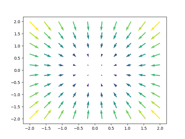
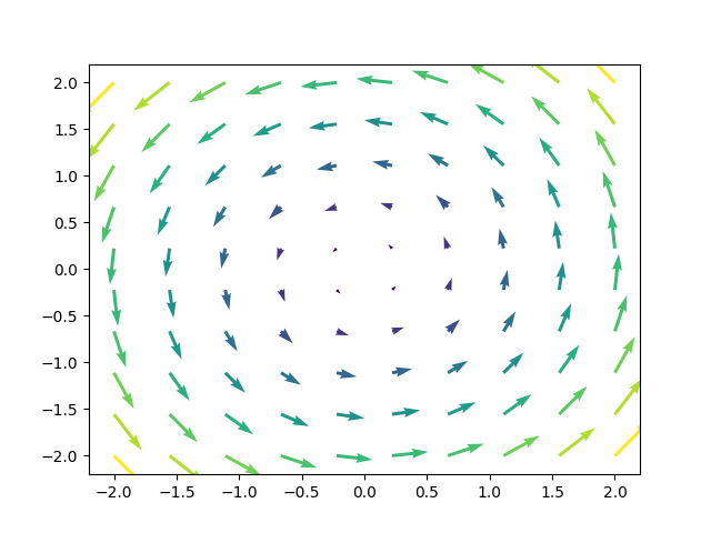
Here are some really good examples of vector fields (Note: we draw just some of the vectors, but really there are vectors associated with every point):
Some things you might care about measuring about a vector field are
- it’s “divergence” at a point: e.g. how much fluid is leaving this point? is the point a source / sink?
- it’s “curl” around a point: e.g. how much is fluid circulating around this point?
Things you might want to measure about functions include - The “gradient” at a point: what is the direction of steepest ascent in function values?
The divergence, \(\nabla \cdot F\), is defined for \(F = (a,b,c)\) as \(\nabla \cdot F = \frac{\partial a}{\partial x} + \frac{\partial b}{\partial y} + \frac{\partial c}{\partial z}\) So for \(F(x,y) = (x,y)\) this is \(2\), and for \(F(x,y) = (-x,-y)\) this is \(-2\) and for \(F(x,y) = (-y,x)\) this is \(0\). This is pretty good, positive divergence means stuff is going out (net), negative divergence means stuff is coming in (net), and zero divergence means stuff is exiting and entering at equal rates.
We can define curl \(\nabla \times F\), for \(F = (a,b)\) (it’s similar in \(\mathbb{R}^3\), I don’t ahve the motivation to type it though) as \((\frac{\partial b}{\partial x} - \frac{\partial a}{\partial y})\vec{k}\).
This gives the zero vector for \((x,y)\) and \((-x,-y)\), and it gives \((0,0,2)\) for \((-y,x)\) (the magnitude is magnitude of curl, and direction of vector indicates clockwise / counterclockwise). (note: the direction is basically determined by the right hand rule from physics).
We can define the gradient of a function \(f\) as \(\left(\frac{\partial f}{\partial x}, \frac{\partial f}{\partial y}, \frac{\partial f}{\partial z} \right)\). For example the gradient of the function \(f(x,y) = x^2 + y^2\) is \(\nabla f = (2x, 2y)\), i.e. you want to go radially outward for steepest ascent.
Remark. Shout out to gradient descent! If you have some parameters \(\Theta\) in some model, and you want to upate your parameters to minimize a cost function \(J\), you basically just do \(\Theta' = \Theta - \alpha \nabla J(\Theta)\). Yay machine learning. (Note: ML is kinda more complex than I’m making it out to be here…)
Anyways, so there are these things– “div, grad, curl and all that” (yes this is the title of a book) – but this all seems kind of physicsy and \(\mathbb{R}^3\) specificy.
We can do better. Let’s do it.
Vector Calculus, Math Edition
OK, so now we’re going to introduce differential forms. This will consist of - defining a differential form - saying how to integrate a differential manifold over some surface - defining the exterior derivative - stating and hand waving about stokses’ theorem
Lets do it.
Definition. Differential form
A differential k-form is a function that takes as input an “anchored k-parallelpiped”, i.e. a point and k spanning vectors for a parallelpiped, and outputs a real number.
A differential 0-form is a nice function
A differential 1-form on, say, \(\mathbb{R}^4\), looks something like this: \(x_1^2 dx_2 + x_3 dx_3\)
How do you evaluate it if you are given an anchored 1-parallelpiped (i.e. a line segment)? Well, let me define the behavior of the basis elements for the vector space of 1-forms on \(\mathbb{R}^4\):
\(dx_i\) extracts the \(i\)-th component from a vector
OK, how does this help? Because I want differential forms to be bilinear functions. Why? well just wait a sec, let me define 2-forms first.
2-forms look like this: \(2x_3dx_1\wedge dx_2\) how do you evaluate one of these? You feed a 2-form 2 vectors, then \(dx_i\wedge dx_j\) extracts the \(i\)-th and \(j\)-th rows of the vectors and then you take the determinant of that matrix, and then you scale by whatever function was multiplying the differential form, evaluated at the anchor point.
In general, a basis k-form on \(\mathbb{R}^n\) looks like say \(dx_{i_1} \wedge \cdots \wedge dx_{i_k}\), and if you feed it \(k\) vectors and an anchor point it will take a \(k\times k\) determinant of the matrix you get by taking rows \(i_1, i_2, \ldots, i_k\) of the spanning vectors.
OK, so because k-forms are defined in terms of determinants (or at least that’s how I defined them, actually you can define determinants in terms of wedge products, and I guess that’s better because you don’t have to chose a basis and stuff, basically you consider a free group of stuffs, and cross out stuff by modding out by the properties that you want like bilinearity and antisymmetry, but anyways I think this coordinate-y definition is maybe more accessible), they inheret this bilinearity and antisymmetry properties.
OK cool, but what’s that weird wedge symbol? Well previously you could have just thought about it as some formal opperator, and \(dx_1\wedge dx_2\)
Definition. Wedge Product
you have 2 forms and you wedge them
its anticommutative, and a linear function of any of the arguments
Definition. Exterior Derrivative
for a function \(f\), it is simply \(\sum_{i=1}^n \frac{\partial f}{\partial x_i} dx_i\)
\(ddf = 0\)
Definition. integral of differential form over a parameterized surface
Say you wanna integrate a form \(\phi\) over a surface \(R = \gamma(I)\), then you have
\[\int_R \phi = \int_{I} \phi_\gamma(D\gamma) dV\]
Theorem. Stokes
\[\int_R \phi = \int_{\partial R} d \phi\]