Rand: “The shortest distance from a point to a line is the perpendicular to the line. Right?”
Alek: “Define shortest, distance, point, line and perpendicular.”
Rand: “Fair engouh…”
Plan:
- Motivating Pictures
- Background
- Linear Algebra: vector space, sub-space, span
- Analysis: norm, distance, convergence, open / closed, inf
- Functional Analysis Definitions: Banach Space, inner product, Hilbert Space
- Projection Theorem
Motivating Pictures
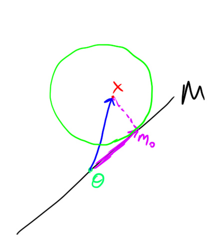
Remark. A natural question in geometry: Given a (suitably nice) region \(M\) and a point \(x \not\in M\) what is the “best” approximation to \(x\) in \(M\)?
In \(\mathbb{R}^2\) with the standard Euclidean norm (e.g. \(||(x,y)|| = \sqrt{x^2 + y^2}\)), if \(M\) is a line (through the origin) then the best approximater
- exists
- is unique
- and satisfies that the error of the best approximator is perpendicular to \(M\)
just as basic geometric intuition tells us (“the shortest distance between a point and a line is perpendicular to the line”). It turns out that we can extend this to some much more general contexts.
Example. Here is a depiction of this optimization problem in \(\mathbb{R}^2\):
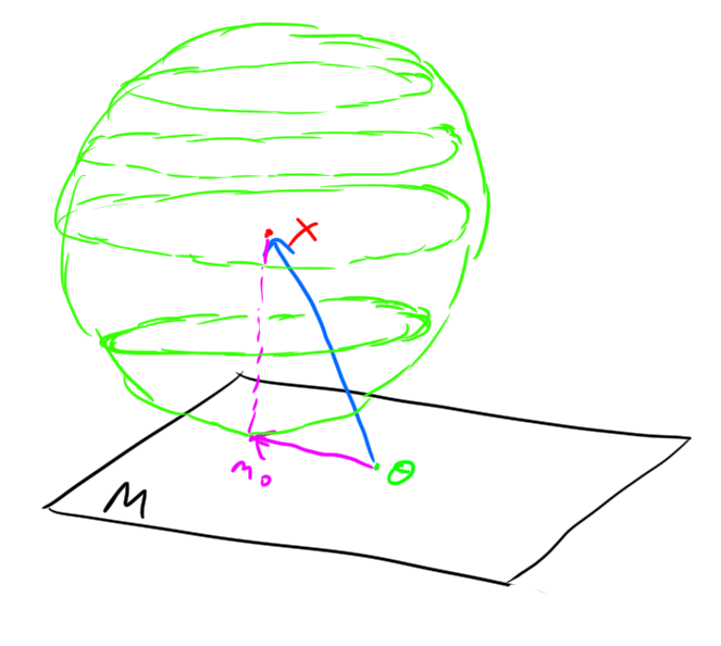
Example. And the optimization problem in \(\mathbb{R}^3\):
Background
Before getting into the functional analysis which will give us the mathematical tools to extend the above geometrical idea,
Linear Algebra
What’s a vector? Some standard definitions:
- “A magnitude and a direction”
- problem: What’s a direction in \(\mathbb{R}^4\)? How about in the space of square summable sequences? The best definition of direction is a vector, so definition of a vector from direction seems circular.
- “A list of n numbers”
- problem: This doesn’t work very well for infinite dimensional spaces.
- “An element of a Vector Space”
- This is the definition that I’ll use, so now I should define vector space (non-circularly).
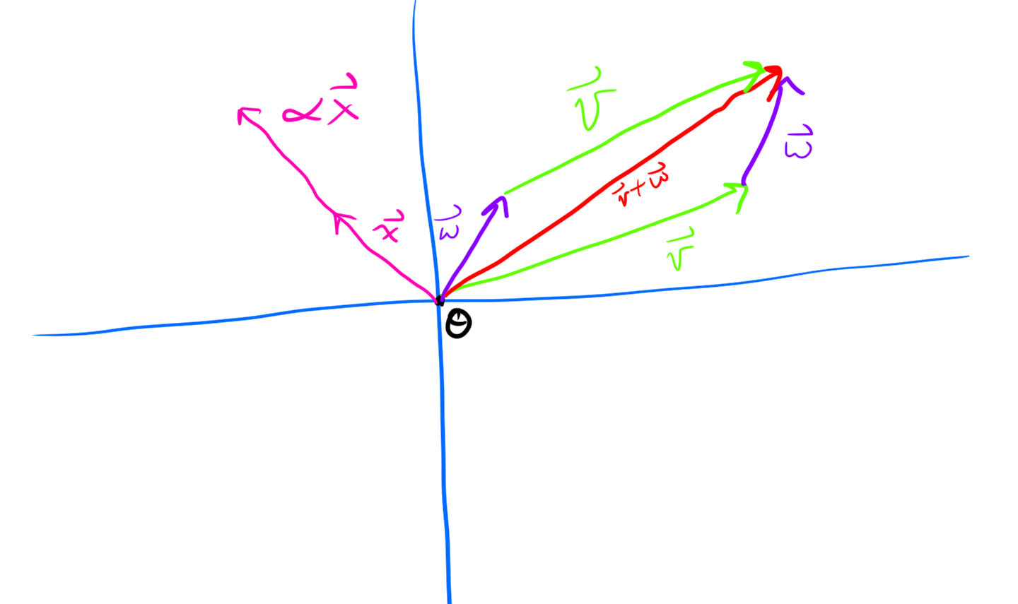
Definition. Vector Space:
We say that a set \(V\) is a vector space over \(\mathbb{R}\) with zero-vector \(\theta \in V\), if for arbitrary \(v, w, x \in V, \alpha, \beta \in \mathbb{R}\) \[\alpha v + \beta w \in V\] \[v+w = w+v\] \[(w+v)+x = w+(v+x)\] \[\alpha(v+w) = \alpha v + \alpha w\] \[(\alpha+\beta) v = \alpha v + \beta v\] \[\theta + x = x\] \[0x = \theta\] \[\exists -x \text{ such that } -x + x = \theta\] \[1x = x\] \[(\alpha\beta)x = \alpha(\beta x)\]
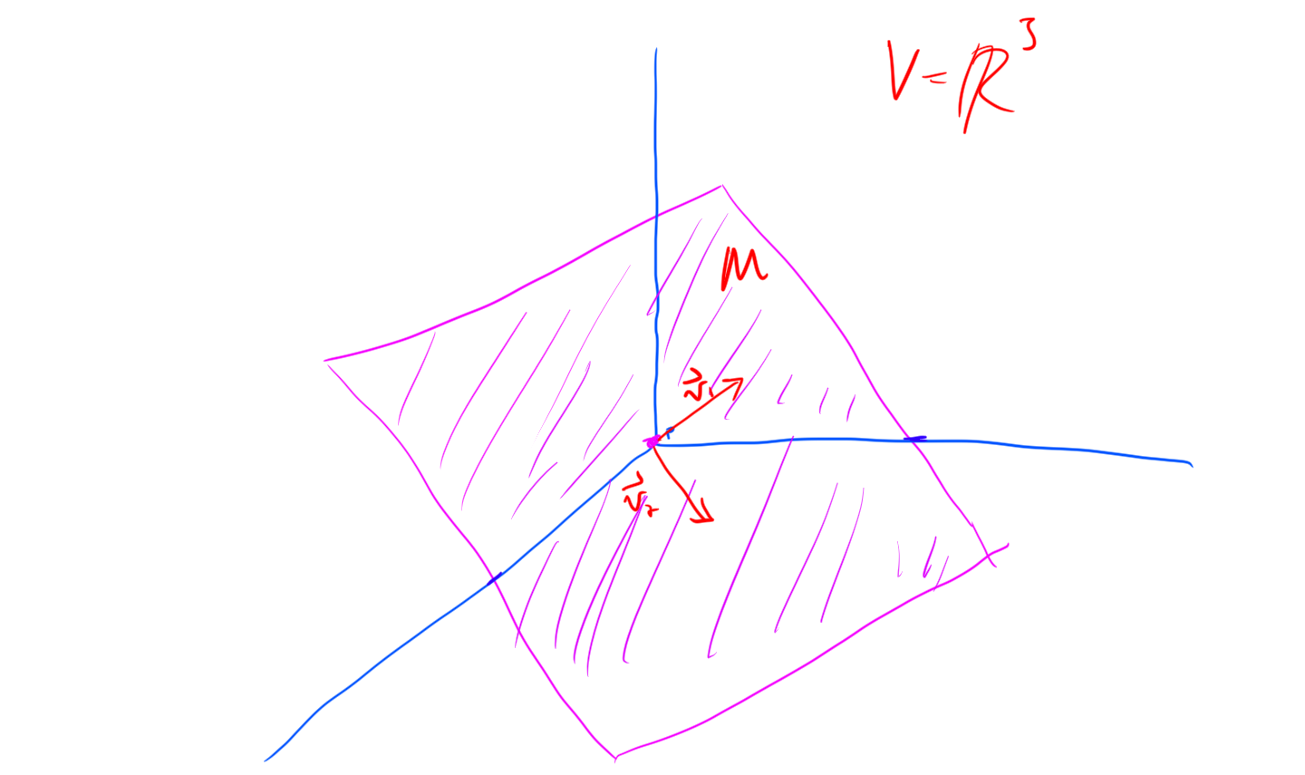
Example. The standard finite dimensional example of a vector space is \(\mathbb{R}^n\).
Definition. \(M \subset V\) is a subspace of \(V\) if \(M\) is closed under linear combinations, that is, \[\forall \alpha, \beta \in \mathbb{R}, x, y \in M, \quad \alpha x + \beta y \in M\]
Remark. Note that \(\theta \in M\) if \(M\) is a subspace. The smallest subspace is the set composed of just \(\theta\), it has dimension \(0\). Note that \(V\) is always a subspace of itself (We say proper subspace if we want the subspace to not be the whole space).
Remark. In \(\mathbb{R}^n\) all subspaces (including the whole space) are expressible as the set of all finite linear combinations of some set of “basis vectors” of size \(\leq n\).
Definition. The span of a set of vectors is the set of all finite linear combinations of these vectors. Equivalently, the span of a set of vectors is the smallest subspace containing all the vectors that it is supposed to span.
Remark. At this point we have the structures of addition of vectors and scalar multiplication. This gives us some geometry, but we are still missing one very important concept… that of size.
Analysis
Definition. (Norm) A norm on a Vector space \(V\) is a funciton \(||\cdot|| : V \to \mathbb{R}\) satisfying
- Positive definiteness: \(||x|| \geq 0 \forall x \in V, \quad ||x|| = 0 \iff x = \theta\)
- Homogeniety: \(||\alpha x || = |\alpha| ||x|| \forall \alpha \in \mathbb{R}, x \in V\)
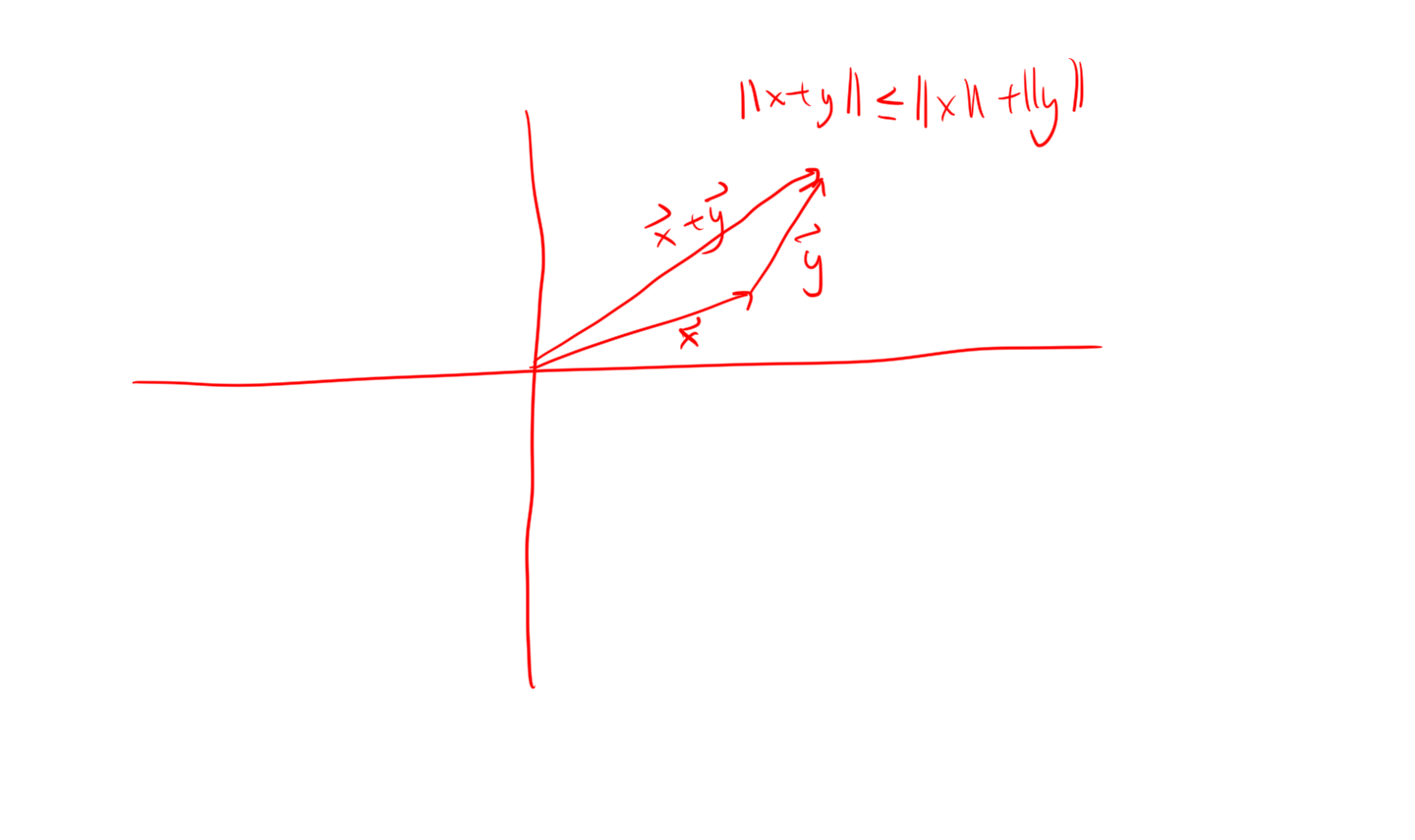
- Triangle Inequality: \(||x+y|| \le ||x|| + ||y||\)
Remark. Recall that the Euclidean norm on \(\mathbb{R}^n\) is defined to be \[||(\xi_1, \ldots, \xi_n) || = \sqrt{\left(\sum_{i=1}^n \xi_i^2\right)}\] Note that the euclidean norm on \(\mathbb{R}^n\) satisfies the axioms for a norm (the triangle inequality is the only non-trivial one to verify, first prove Cauchy Shwarz).
Definition. We call a Vector space \(X\) along with a norm \(||\cdot ||\) a normled linear space.
Definition. The distance between 2 vectors \(x, y \in X\) is defined to be \[|| x- y ||\]
Definition. A sequence \((x_n)_{n=1}^\infty \in V\) converges to a value \(x \in V\) iff \[\forall \epsilon > 0, \exists N \text{ such that } \forall n> N \quad ||x_N - x|| < \epsilon\] or more simply put, eventually the sequence values stay arbitrarily close to the limiting value. Also equivalently, for every ball around \(x\), only finitely many terms of \(x_n\) lie outside the ball.
Definition. A sequence \((x_n)_{n=1}^\infty\) is Cauchy iff \[\forall \epsilon > 0 \exists N \text{ such that } m, n > N, ||x_n - x_m|| < \epsilon\] Here the terms are getting arbitrarily close to one another.
You might guess that convergence and Cauchy are equivalent, but this isn’t quite true in general… The problem is that your space might have “holes” in it. If your space is complete then this is not an issue.
Definition. A space is complete if all Cauchy sequences in it converge in it
Example. \(\mathbb{R}\) is complete
Remark. \(\mathbb{Q}\) is not complete! For example, the sequence of decimal approximations of \(\pi\) is Cauchy, but doesn’t converge in \(\mathbb{Q}\) i.e. doesn’t converge to a rational number.
Definition. Given a normed linear space \(X\), a set \(K \subset X\) is said to be closed if all cauchy sequences in it converge. (the set is closed under limits).
Example. For example, the set \[\{ (x,y) : x^2 + y^2 \leq 1 \}\] is a closed set in \(\mathbb{R}^2\).
For non-example, the set \[\{ (x,y) : x^2 + y^2 < 1 \}\] is not a closed set in \(\mathbb{R}^2\) (in fact its complement is closed, so it is called an open set).
Definition. The infimum of a set of real numbers, denoted \(\inf S\) is the greatest lower bound for \(S\). That is, all \(x\in S\) satisfy \(x \geq \inf S\), and also, \(\forall \epsilon > 0\) \(\inf S + \epsilon\) is not a lower bound, so \(\exists s \in S\) such that \(\inf S \leq s < \inf S + \epsilon\).
Functional Analysis Definitions
Now I’ll use the ideas from linear algebra and real analysis to develop discuss some examples of normed linear spaces.
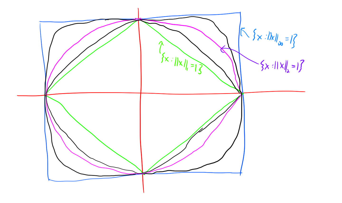
Just by varying the norm we get interesting different normed linear spaces. In \(\mathbb{R}^2\) the standard norm is the map \((x,y) \to \sqrt{x^2 + y^2}\), but another reasonable norm is the “taxicab norm” \((x,y) \to |x| + |y|\) (interpret this as: if you have to travel parallel to the axes, then the shortest distance between 2 points is the number of units along the x axis you must travel plus the number of units along the y axis you must travel). Another norm that could be interesting is the map \((x,y) \to (|x|^3 + |y|^3)^{1/3}\) (motivation: volumes…). We can define the following general class of norms:
Definition. The \(p\)-norm of a list is defined to be: \[||(\xi_1,\xi_2,\ldots)||_p = \left(\sum_{i\geq 1} |\xi_i|^p \right) ^ {1/p}.\] This definition works for \(p \in [1,\infty)\), there is an \(\infty\)-norm too, which is in a sense the limit as \(p\to \infty\) of the other \(p\)-norms, but for completeness ( ;) ) it is defined separately as \[||(\xi_1, \xi_2, \ldots)||_\infty = \sup_{i\geq 1} |\xi_i|\]
Note that I don’t specify that this is a finite list. This is because the \(p\)-norm can be applied to infinite lists just as it is applied to finite lists. This prompts the definition of a space of infinite sequences:
Definition. \(\ell^p\) is the space of infinite sequences \((\xi_1, \xi_2, \ldots)\) that satisfy \[||(\xi_1, \xi_2, \ldots)||_p < \infty\] So any element of \(\ell^p\) has to have finite \(p\)-norm. If we endow \(\ell^p\) with the \(p\)-norm we get a normed linear space.
Proposition. \(\ell^p\) with the \(p\)-norm is a Banach space
This is a tough one to prove. You need to prove Holder’s inequality first to even show that the functional I defined is a norm, and completeness is rather subtle. I might add this proof later.
Remark. Drawing the unit balls for \(\mathbb{R}^2\) with the different \(p\)-norms is really informative.
OK, so far the dimension of our vector spaces has been countable. Lets get bigger! Function vector spaces are really big.
An analogy to the \(p\)-norm for lists is the following for functions:Definition. The \(p\)-norm for functions is \[\left(\int_0^1 |x(t)|^p dt \right)^{1/p}\] and the \(\infty\)-norm is \[\text{ess sup}_{t\in [0,1]} |x(t)|\]
Definition. \(L^p([0,1])\) is the space of functions on \([0,1]\) that satisfy \[||x||_p < \infty\]
Remark. OK fine not quite. This wouldn’t quite work, because any function that differs from the 0 function on a set of measure 0 would have norm 0 violating the norm axiom that only the 0 vector can have norm 0. The solution is to consider equivalence classes of functions. Functions are equivalent if they differ on a set of measure 0.
There is one extra piece of geometry that would be nice, namely an inner product. This is the straightforward generalization of the dot product in \(\mathbb{R}^2\)
For sequences this is defined asDefinition. Let \(x = (\xi_1, \xi_2, \ldots), y = (\eta_1, \eta_2, \ldots) \in \ell^2\), then we define the inner product as \[(x | y) = \sum_{i\geq 1} \xi_i \eta_i\]
Definition. \[(x|y) = \int_0^1 x(t) y(t) dt\]
Remark. Note the similarity between the definitions, the idea is that we point-wise / component-wise multiply the functions / sequences and then “sum” this.
Proposition. The inner product is
- Bilinear: \((\alpha x + \beta y | z) = \alpha(x | z) + \beta (y | z)\)
- Symetric: \((x|y) = (y|x)\)
- Positive definite: \((x|x) \geq 0\), \((x|x) = 0 \iff x = \theta\)
Why don’t we define this for any Banach space? Because it is nice when the inner product induces the norm, and this only happens in \(\ell^2\) and \(L^2\).
Remark. The sense in which the inner product induces the norm is that \[(x|x) = ||x||_2^2\]
Definition. A normed linear space where the norm is induced by an inner product on the space is called a Hilbert space.
The geometry that the inner product gives us access to is the notion of orthogonality.
Definition. Vectors \(x,y\) are said to be orthogonal iff \[(x|y) = 0\]
Orthogonality makes possible the notion of projection.
Proof of Projection Theorem
Theorem. Let \(H\) be a Hilbert space, Let \(M\subset H\) be a closed subspace, let \(x \in H\). Then, there exists a unique \(m_0\) satisfying \[|| x - m_0 || = \inf_{m \in M} || x - m ||\] and \(m_0\) is characterized by \[x-m_0 \perp m \quad \forall m \in M.\]
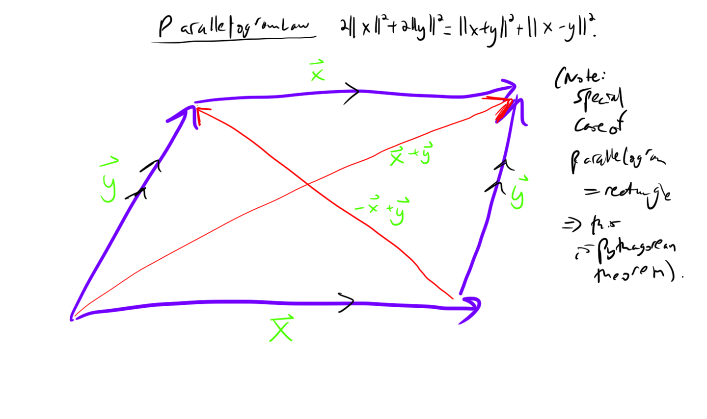
Lemma. By bilinearity and symmetry: \[||x - y||^2 + ||x+y||^2 \] \[= (x-y | x-y) + (x+y | x+y) = 2(x|x) + 2(y|y) = 2||x||^2 + 2||y||^2\] This is actually a theorem from geometry, the “parallelogram law”.
Now, I’ll prove the projection theorem. The proof strategy is as follows:
- Fisrt I will exhibit a sequence which converges to \(m_0\)
- Then I will show that \(m_0\) is unique
- Finally I will show that orthogonality of error characterizes \(m_0\)
Proof.
Exhibit a sequence that converges to \(m_0\):
The \(\inf\) naturally gives rise to a sequence, namely the sequence induced by the fact that any number larger than the \(\inf\) fails to be a lower bound, so there exists a term which violates any greater attempt at a lower bound.
Let \(d = \inf_{m\in M} ||x-m|| > 0\) Then \(\forall \epsilon > 0\), \(\exists m_\epsilon \in M\) such that \(||x-m_\epsilon|| < d + \epsilon\).
Take \(\epsilon = 1/n\) to generate a sequence \((y_n)_n\) in \(M\).
We now show that this sequence is cauchy:
Note that by the Parallelogram Law (see above lemma) \[||y_n - y_m||^2 = ||(y_n - x) - (y_m - x)||^2 \] \[\le 2||y_n - x||^2 + 2||y_m-x||^2 - ||(y_n-x) + (y_m -x)||^2\] \[= 2||y_n - x||^2 + 2||y_m-x||^2 - 4||\frac{1}{2}(y_n + y_m) - x||^2\]
And, critically, \(\frac{1}{2}(y_n + y_m) \in M\) (because \(M\) is a subspace, and so closed under finite linear combinations), so we have, by definition of the \(\inf\), \[||\frac{1}{2}(y_n + y_m) - x ||^2 \geq d^2.\] Combining this with the above inequality we have, \[||y_n - y_m||^2 \le 2 ||y_n-x||^2 + 2||y_m-x||^2 -4d^2. \]
Now, because \(||y_k - x|| \to d\), for any \(\epsilon > 0\) \(\exists N\) such that \(\forall n,m > N\), \[||y_n - y_m||^2 \le 2 d^2 + \epsilon/100 + 2d^2 + \epsilon /100 -4d^2 < \epsilon.\] Hence the sequence is convergent.
Prove uniqueness of \(m_0\):
This is actually quite easy. Let \(m'\) also be a minimizer. Then the sequence \(y = m_0, m', m_0, m', \ldots\) is a sequence that has \(||y_n -x|| \to 0\) (trivially, because \(||y_n - x|| = 0\) \(\forall n\)), and by the above proof this implies that \(y\) is Cauchy. That is, \(||y_n - y_m||\) gets arbitrarily small as \(m,n\to \infty\). This implies that \(||m' - m_0 || = 0\), hence \(m_0 = m'\).
Orthogonality of error characterizes \(m_0\):
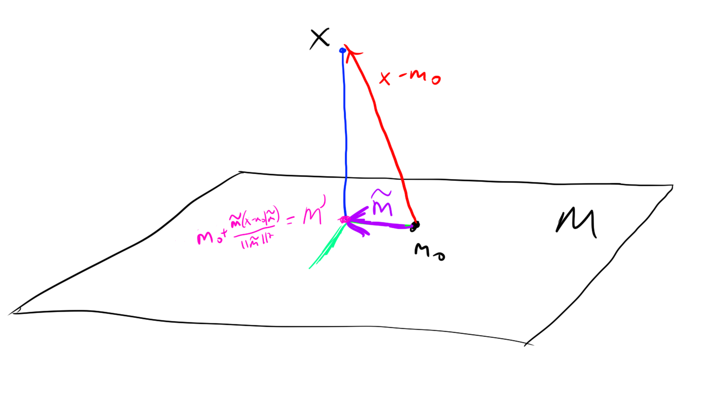
Assume for contradiction that \(x - m_0 \not \perp \tilde{m}\) for some \(\tilde{m} \in M\). WLOG \(||\tilde{m}|| = 1\) (because given any \(\tilde{m}\) we could scale it to be a unit vector, and we are in a subspace, which is closed under this scaling.) Also WLOG \((x-m_0 | \tilde{m}) > 0\) (if it is negative we multiply \(\tilde{m}\) by \(-1\)).
Then we construct a new candidate minimum that will contradict the assumed minimality of \(\tilde{m}\) as follows: \[m' = m_0 + \tilde{m} (x-m_0 | \tilde{m}) \] The picture suggests why this is a good new candidate minimizer, we essentially are projecting some of the error into the subspace, and then moving to remove the error, so it makes a lot of sense that \(||m' - x|| < ||m_0 - x||\). Here is the proof of this observation:
\[|| x - m' ||^2 = (x-m' | x-m') \] \[ = (x - m_0 - \tilde{m} (x-m_0 | \tilde{m}) | x - m_0 - \tilde{m} (x-m_0 | \tilde{m})) \] \[ = ||x - m_0||^2 -2(x-m_0 | \tilde{m} (x-m_0 | \tilde{m})) + ||\tilde{m} (x-m_0 | \tilde{m})||^2 \] \[ = ||x - m_0||^2 -2 (x-m_0 | \tilde{m})^2 + (x-m_0 | \tilde{m})^2 \] \[ = ||x - m_0||^2 -(x-m_0 | \tilde{m})^2 \] \[ < ||x - m_0||^2. \]
This shows that if the error is not orthogonal, then the vector is not the optima (thus the contrapositive is true, for the optima, the error is orthogonal to \(M\)).