The Probabilistic Method
preface
I am going to try to read “The Probablistic Method” by Noga Alon and Joel H. Spencer. The Probablistic Method, pioneered by Erdos, is a really interesting way to think about combinatorics problems. Here is a high level overview of how proofs by the probabilistic method go
Consider a random thing
Break the thing up into simple sub-things
Compute something on the sub-things
Combine the sub-things together to get
Pr[thing is good] > 0
Thus, there must be some thing that is good.
The approach is often pretty non-constructive but sometimes it can be made constructive.
resonable example
Remark. Yup I’m putting math in the preface to my blog! I think this is a good idea. It gives you a bit of a better idea what this blog is about. It’d be kind of weird to keep reading for hours before you even know what the probabilistic method is!
Let \(\mathcal{F}\) be an intersecting family of sets Let \(2k \le n\) and suppose \(\mathcal{F}\) is an intersecting family of \(k\) element subsets of an \(n\) set
Theorem. “Erdos-Ko-Rado Theorem” \[|\mathcal{F}| \le {n-1 \choose k-1}\]
Remark. This is tight! It is achievable by the “sunflower configuration”, where you choose all sets that intersect with \(0\)
Lemma. can contain at most k sets of the form s+[k]
Proof. fix some set \(t+[k]\) in \(\mathcal{F}\). To intersect \(t+[k]\) the set has to be like \(t-i+[k]\) or \(t+i+[k]\) for some \(0 < i < k\). There are \(2(k-1)\) such sets. We can pair off sets of the form \(s+[k]\) with sets of the form \(s+k+[k]\). Because \(2k \le n\) these sets are disjoint. Hence, \(\mathcal{F}\) contains at most one of them. Hence \(\mathcal{F}\) contains at most \(2(k-1)/2 + 1 = k\) of these types of sets.
Proof. (proof of Erdos-Ko-Rado Theorem)
Choose a random permutation \(\pi\) of \([n]\). Choose a random \(i \in [n]\). Conditioning on \(\pi\), the probability of \(\sigma(i+[k]) \in \mathcal{F}\) is at most \(k/n\) by the Lemma (relabel stuff). The probability of A is of course equal to \(|\mathcal{F}| / {n \choose k}\). Thus we have \[\frac{|\mathcal{F}|}{{n \choose k}} \le \frac{k}{n}.\] Hence \[|\mathcal{F}| \le {n \choose k} \frac{k}{n} = {n-1 \choose k-1}.\]
story
Remark. This part is a somewhat soggy and crumbly “personal motivation for doing this story thing”. Consider skipping straight to my post on Chapter 0, or even Chapter 1. Nevertheless I feel obligated to write an at least somewhat compelling preface, because I like to read prefaces. So yeah, whatever. If the real numbers are complete, then I better be complete in my blogging.
I want to read this book because I believe that it contains some really elegant math, and I think math is super cool. The first half of my senior year wasn’t super fun for me; I was super busy and doing a lot of things that I didn’t find very interesting. Thinking back on that time, the most prominent positive memory is of math. In particular, I was taking a functional analysis class. Twice a week, every week, I would rush out of school and jump on my bike to ride over to a local university (Harvard) where I was listening to the lectures. I left behind all the baggage of tasks performed grudgingly and was immersed in theland of infinite dimensional vector spaces and bounded linear functionals for a magnificent hour and fiveteen minutes. On weekends and whatever other spare moments of time that I found I worked on the psets for the class, which usually consisted of a couple really interesting and often pretty challenging proofs.
One time when I was biking there it rained (really hard). Prior to the bike ride I was annoyed because of “school and stuff”. I was completely soaked by the time I got there, and pretty cold too (Note: some people have pointed out that I should have taken the bus instead of biking, especially when the weather was sub-optimal. This is a good point. Also note that I am not advocating for biking in the rain, especially when it is cold. In fact this is kind of a dumb thing to do.). Yet, seemingly strangely I felt very happy while biking. I thought about it a bit and came up with this list of things that I think made my experience with functional analysis so great:
- I was learning it purely for fun (in particular, I didn’t tell my school that I was taking this class, and didn’t do anythign with my grade)
- An incredibly enthusiastic professor guided us through the definitions and proofs from the book, with many fun examples (on a black board!)
- The content had some really interesting and non-trivial, while still elegant, proofs.
- I was able to share the novel math I was learning with my friends. I did this a lot while walking to and from school, and I also gave a talk to our math team about it and even wrote a (short) blog post about it!!!
Anyways, this story does have a point. It just is going to take me a minute to get to it.
The point is: I love math.
OK, you might say, I probably could have guessed that. What’s with the long story?
I love math, But keeping a consistent schedule, even at doing things that you love, is hard (for me at least), especially if the thing in question is challenging. Other stuff will innevitably try to get in the way. That’s where this blog comes in. I’m going to write a blog post regularly about the chapter of the Probabilistic Method that I’ve been reading. Having a blog means that with non-zero probability some people will be sad if I don’t read for a week. It also gives me a very nice record of the things I’ve learned, and will look very cool (I plan to draw lots of pictures). So that’s my selfish rationale for writing this blog.
Furthermore, maybe this blog can teach you some cool combinatorics too! I will do my best to make my explanations compelte and understandable to people who haven’t been reading the book. In particular I will introduce any combinatorial objects that it talks about. Sharing math with others is something I find super fun, so I hope you enjoy.
If you’re interested in reading this, please don’t be put off by all the fancy words and stuff, or by personal feelings of inadequacy. I didn’t know what a “Ramsey number” or a “Hypergraph” was before reading this book either. In actuality these are not too complicated ideas; I hope to be able to convince you of this proposition by drawing some pictures. Some more notes:
- If you read this and think it’s cool please let me know!
- If you read this and are confused about something, also let me know! I’d love to talk about it!
- If you read this and think I’ve botched some math somewhere, definitely let me know!
A final note to the reader: this blog is going to be somewhat casual, especially in terms of language used, although also sometimes in terms of definitions and proofs. In particular I’m potentially gonna use slang, and exclamations of excitement such as “yo epic” and “now that’s pretty cool” or similar. Also there are going to be a lot of speelling mistakes. I hope neither of these things distract from the mahtematical content of the blog (in fact I suspect the enthusiasm will be helpful).
Really the final note to the reader before starting:Remark. Thank you for reading! (conditional on the existence of you). I hope you find this experience as epic as I have.
Now we begin our discussion of THE PROBABILISTIC METHOD!!!!!!
Chapter 0
[[May 13]]
This is not a chapter in the book. In this post I’m just going to define a bunch of combinatorial objects. Some of them you are likely already familiar with, but some definitions may be new. At least look at the pictures.
some basic combinatorial objects
Definition. A set is an (unordered) collection of distinct objects.
Example. Some nice sets:
- \(\mathbb{N}= \{1,2,\ldots, \}\) (natural numbers)
- \(\mathbb{Z}= \{\ldots, -2, -1, 0, 1, 2, \ldots \}\) (integers)
- \(\mathbb{Q}= \{ p/q : p,q\in \mathbb{Z}, q\neq 0 \}\) (rationals)
- \(\mathbb{R}\) is the completion of \(\mathbb{Q}\) (reals)
- \(\mathbb{R}^n\)
- \(\mathbb{C}\)
- \([n] = \{1,2,\ldots, n\}\)
- \(\{\{1,2\}, \{1,2,3\}\}\)
- \(\{(1,2), (2,3)\}\)
Remark. You might notice that I didn’t list the ZFC set theory axioms. That’s because
- this is a blog post on combinatorics
- basically all the sets we are going to be dealing with are finite
- I don’t know a lot about set theory
Definition. A multiset is an unordered collection of possibly not distinct objects
Example. some multisets:
- \(\{1,2\}\)
- \(\{1,1,1,2\}\)
Definition. An \(n\) element list, also called a \(n\)-tuple, is an ordered set of elements
Example. some lists:
- \((1,2,3,4,5)\)
- \((5,4,3,2,1)\)
Definition. An undirected graph is composed of a set \(V\) of “vertices” along with a set \(E\) of “edges”. Every edge \(e \in E\) is composed of 2 vertices, i.e. \(e=\{x,y\}\) for vertices \(x, y \in V\).
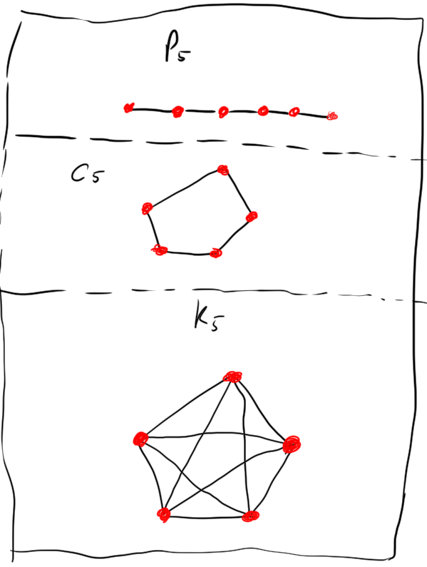
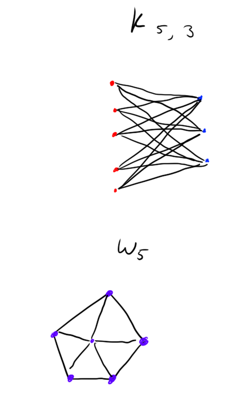
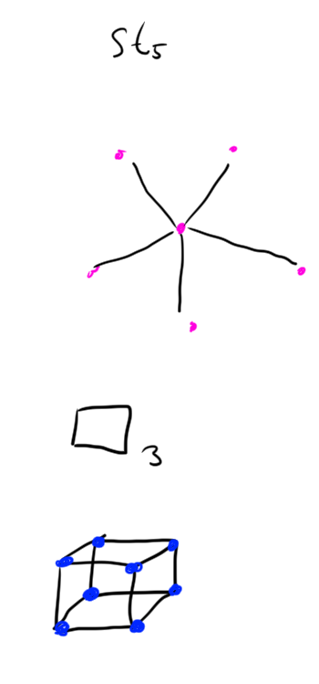
Example. See graphical depictions of these graphs below. (vertices are represented by dots, edges by lines)
- \(P_n\) the path graph with \(n\) edges.
- \(C_n\) the cycle graph on \(n\) vertices.
- \(K_n\) the complete graph on \(n\) vertices
- \(K_{n, m}\) the complete bipartite graph with one part having \(n\) vertices, and the other part having \(m\) vertices.
- \(W_n\) the wheel graph on \(n\) vertices.
- \(St_n\) the star graph on \(n\) vertices.
- \(\square_n\) the cube graph in \(n\) dimensions.
(thanks to this random site for their “dictionary of graphs” )
Definition. A directed graph is a composed of a set \(V\) of vertices along with a set \(E\) of edges. Here the edges are directed, i.e. they are lists rather than sets. e.g. \((x,y) \in E\) for \(x,y\in V\) is an edge.
Example. 
Definition. A tournament on \(n\) vertices is a orientation of the edges in \(K_n\). That is, for each pair of distinct \(x, y \in V\) either \((x,y) \in E\) or \((y, x) \in E.\)
Example. 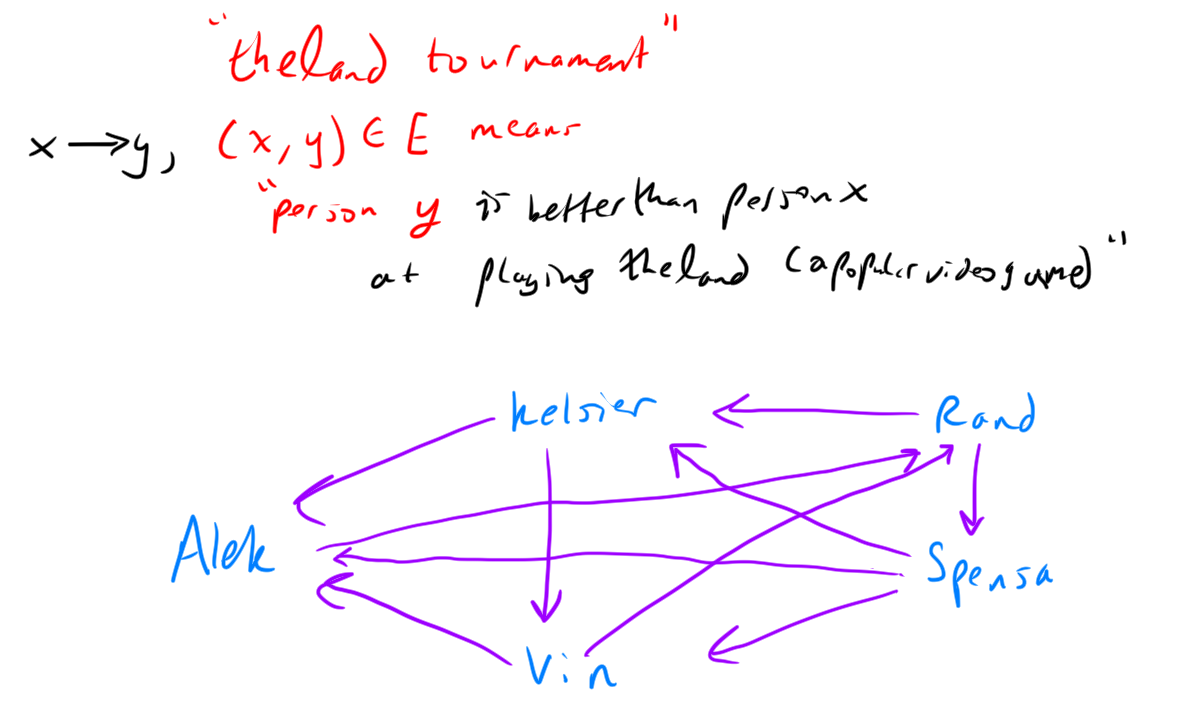
Definition. A hypergraph is a set of vertices \(V\) along with a family \(E\) of subsets of \(V\) called edges.
Example. 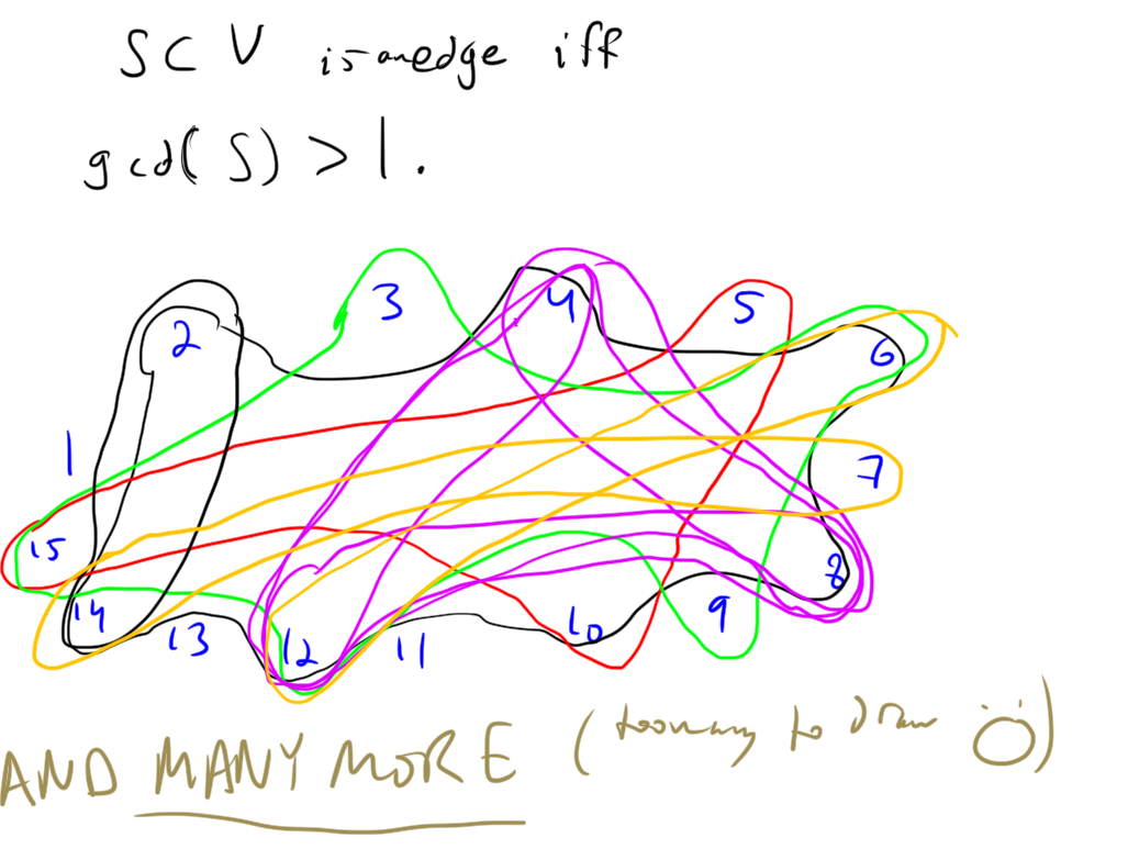
some basic functions
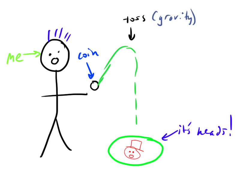
Definition. Without getting into measure theory, here’s my shot at defining / describing a random variable.
“The outcome of a random process”
Example.
- A fair coin toss (aka Bernouli random variable with \(p=1/2\))
- Flip \(100\) coins, count number of heads (aka binomial random variable with \(p=1/2\), \(n=100\))
Definition. Probability distribution. For the discrete case these are probability mass functions. In the continuous case we need probability density functions.
Assigns probabilities to events.
Probabilities are non-negative, and should sum/integrate to \(1\).
Example. some pmfs:
- \(\Pr(X=k)= 1/n\) for \(k \in [n]\). (uniform distribution on \([n]\))
- \(\Pr(X=k) = p^k (1-p)^{n-k} \binom{n}{k}\) for \(k \in 0,1,\ldots, n\) (binomial PMF with parameters \(n, p\))
- \(\Pr(X=k) = \frac{e^{-\mu} \mu^k}{k!}\) for \(k=0,1,2,\ldots\) (poisson PMF with parameter \(\mu\))
Definition. An event is a subset of the possible things that can happen.
Example.
- You flip 2 coins and get at least \(1\) head.
- You choose a random number uniformly from \([0,1]\) and it is at most \(0.1415\).
Definition. The expectation of a random variable \(X\) is
\[\mathop{\mathrm{\mathbb{E}}}[X] = \sum_{x} x \Pr(X=x)\]
this is just “weighted average of outcomes using probabilities as weights”
Example. Some examples
- If you flip \(100\) coins the expectation of the random variable “number of heads” is \(50\)
OK, sorry if these definitions are a bit too soggy and non-rigorous for the measure theory enthusiasts / people who know about probability. Also sorry if it is too long and you’re bored now, or if its too short and I forgot to define important things. Luckily you can google stuff. Anyways, see you next chapter!!
Chapter 1
[[May 13]]
(yes I’m writing these concurrently. gotta jump start the blog.)
OK!!! We’re going to actually show the probabilistic method in action now, through a very cool example: Ramsey Numbers.
Definition. The Ramsey Number \(R(a,b)\) is the smallest number of people that must be in a room such that there must be either a subset of \(a\) people who all know each other or a subsetof \(b\) people who all don’t know each other.
Here are two more “graph-theoretically-technical” ways of saying this.
\(R(a,b)\) is the minimum \(n \in \mathbb{N}\) such that any graph on \(n\) vertices must either have an \(a\)-clique (i.e. have \(K_a\) as an induced subgraph) or have a \(b\)-independent set (i.e. have a completely disconnected induced subgraph on \(b\) vertices).
\(R(a,b)\) is the minimum \(n\in\mathbb{N}\) such that any \(2\)-coloring of \(K_n\) with red and blue must have a \(K_a\) monochromatic red induced subgraph or a \(K_b\) monochromatic blue subgraph.
Computing \(R(a,b)\) is in fact a large open problem in combinatorics. Very few non-trivial values of this function are known.
Example. Let’s compute some trivial values and bounds on \(R(a,b)\)
- \(R(a, b) = R(b, a)\) because if you swap the colors red and blue then its still the same number.
- \(R(1, c) = 1\) because if you have \(1\) person, then there is definitely \(K_1\) as a subgraph and it’s certainly monochromatic (it has no edges :) )
- \(R(2, c) = c\) because
- if we color every edge in \(K_n\) blue for \(n<c\) then there clearly is no monochromatic red \(K_2\) or a monochromatic \(K_c\) contained in this graph
- But, in \(K_c\),
- Either every edge is blue, in which case there is a monochromatic blue \(K_n\)
- There is a red edge, in which case there is a monochromatic red \(K_2\)
Example. Now we are going to compute the only other value of \(R(a,b)\) that I know how to compute: \(R(3,3)\).
First, note that \(R(3,3) > 5\) by the following picture:
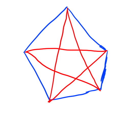
If you look at this graph, you’ll see that there are no monochromatic triangles (\(K_3\)’s). Thus \(n=5\) is not large enough to guarantee that every \(2\)-coloring of \(K_n\) has a monochromatic triangle (\(K_3\)).
On the other hand though, I claim \(R(3,3) \le 6\).
Here’s why: Consider a coloring of \(K_6\) and take some vertex \(v\). \(v\) of course has \(5\) neighbors. By the pidgeon-hole principle \(v\) either has at least \(3\) red edged neighbors or at least \(3\) blue edged neighbors. WLOG let’s say \(v\) has at least \(3\) red edged neighbors.
None of these neighbors can be connected to each other by a red edge, or else they would form a red triangle with \(v\)! But then we are forced to have a blue triangle! So it’s impossible for \(K_6\) to not have a monochromatic triangle.
Thus \[R(3,3) = 6.\]
Now I’m going to derive some cool bounds on the Ramsey numbers. First I’ll derive an upper bound. This proof doesn’t use the probabilistic method, but it’s still cool. I read the proof here.
Theorem. \[R(a, b) \le R(a-1,b) + R(a, b-1)\]
Proof. It’s actually pretty similar to the \(R(3,3) \le 6\) proof.
Let \(n = R(a-1,b)+R(a,b-1)\). Assume for contradiction that there exists a \(2\)-coloring of \(K_n\) (with red and blue) such that \(K_n\) doesn’t have \(K_a\) monochromatic red subgrpah or \(K_b\) monochromatic blue subgraph.
Fix a vertex \(v\). Let \(A\) be the set of neighbors connected to \(v\) with red edges, and \(B\) be the set of neighbors connected to \(v\) with blue edges. There are \(n\) total vertices, so \(|A|+|B|+1=n\).
Now consider the induced subgraph on \(A\). By assumption \(A\) doesn’t contain a \(K_b\) monochromatic blue subgraph. Furthermore, each vertex in \(A\) is connected to \(v\) by a red edge, so if \(A\) has a red \(K_{a-1}\) then there is a red \(K_a\), which cannot be either, also by assumption. Thus we have \(|A| \le R(a-1, b) -1\).
By identical reasoning we have that \(|B| \le R(a, b-1) -1\).
However this is problematic: \[n = |A|+|B|+1 \le R(a-1, b) -1 + R(a,b-1) -1 + 1 = n-1\] a contradiction.
Hence \(K_n\) actually must have a monocrhomatic red \(K_a\) or monochromatic blue \(K_b\). And thus \(R(a,b) \le n\) as desired.
Corollary. \[R(a,b) \le \binom{a+b-2}{a-1}\]
and in particular \[R(k, k) \le O\left(\frac{4^{k-1}}{\sqrt{k-1}}\right).\]
Proof. The recurrence is obviously binomial coefficients. For the base case use the trivial values of \(R(a,b)\) that we computed.
Plugging in \(a=b\) we get central binomial coefficients, which can be estimated easily by Stirling’s approximation.
ok, now what you’ve actually been waiting for the first proof in the book!! a lower bound on diagonal Ramsey numbers by the probabilistic method.
Theorem. Fix \(k\). Let \(n\) be sufficiently small such that \(\binom{n}{k}2^{1-\binom{k}{2}} < 1\).
Then \(R(k,k) > n\) (i.e. there is some \(2\)-coloring of \(K_n\) that doesn’t have any monochromatic \(K_k\) induced subgraphs)
Proof. Let \(n\) be as specified. Consider a random \(2\)-coloring of \(K_n\) with each edge being randomly red or blue with equal probabilities (\(1/2\)) and all these random choices being made independently.
For any set of \(k\) of the vertices (\(S \subset V\) with \(|S| = k\)) let the \(M_S\) be the event that the induced subgraph on \(S\) is monochromatic.
For any \(S\) \[\Pr[M_S] = 2\cdot \frac{1}{2^{\binom{k}{2}}}\] because there are \(\binom{k}{2}\) edges in \(S\), and \(S\) could be monochromatic red or blue.
By the union bound we have
\[ \Pr\left[ \bigvee_{S\subset V, |S|=k} M_S \right] \le \sum_{S\subset V, |S|=k} \Pr[M_S] = \binom{n}{k} 2^{1-\binom{k}{2}} < 1\] by assumption.
But then the probability that all events \(M_S\) do not occur is strictly positive.
Hence for some random \(2\)-coloring it must be that all events \(M_S\) do not occur.
That is, there is some \(2\)-coloring of \(K_n\) for which there are no monochromatic \(K_k\) induced subgraphs.
Corollary. \[R(k,k) > \lfloor 2^{k/2}\rfloor\] for \(k \ge 3\).
Proof. We claim that \(n=\lfloor2^{k/2}\rfloor\) satisfies \(\binom{n}{k}2^{1-\binom{k}{2}} < 1\). Note that \[\binom{n}{k}2^{1-\binom{k}{2}} \le \frac{1}{k!}\frac{2^{k^2/2}}{2^{k^2/2-k/2 -1}} = \frac{2^{k/2-1}}{k!} < 1\] for \(k \ge 3\) because I graphed it.
Remark. Stirling’s approximation says \[k! \sim \sqrt{2\pi k} (k/e)^k\] (i.e. the ratio of these functions tends towards \(1\) as \(n\to\infty\)).
Chapter 2
[[May 13]]
(yes again all this is written on the same day. ok writing this much on one day was probably a bad idea. but it was fun so whatever. I did get a little tired by the end, but I think I stopped before the content started suffering.)
Chapter 2 is about Expectation. Specifically the new proof strategy highlighted looks like this:
make some random thing
Compute the expectation of it
there has to be a point where \(X \ge \mathop{\mathrm{\mathbb{E}}}[X]\) and where \(X \le \mathop{\mathrm{\mathbb{E}}}[X]\)
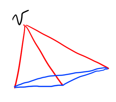
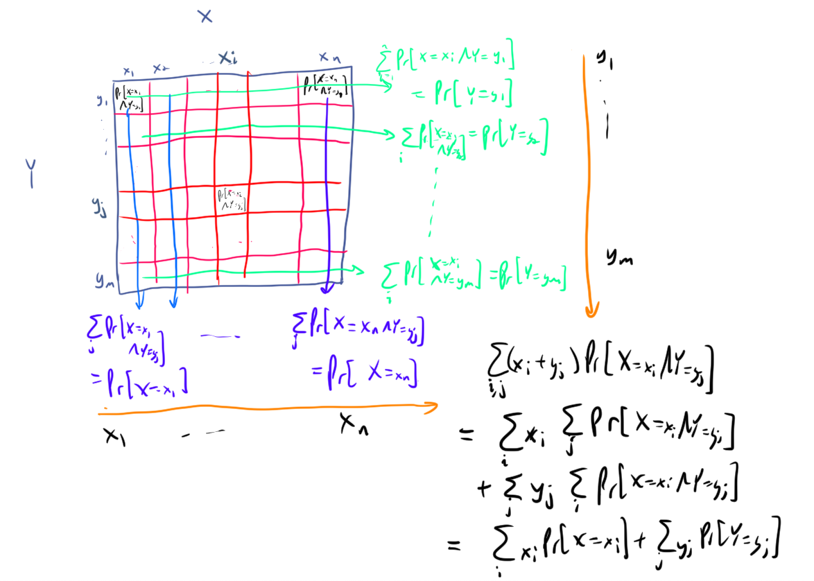
One really nice thing about expectation is that it’s linear. I recently was talking about this with people, and I thought of a really nice picture to go with my usual proof of this fact.
Theorem. Expectation is linear That is, if \(X, Y\) are random variables and \(a \in \mathbb{R}\) is some scalar, then
\[\mathop{\mathrm{\mathbb{E}}}[X+Y] = \mathop{\mathrm{\mathbb{E}}}[X] + \mathop{\mathrm{\mathbb{E}}}[Y]\] and \[\mathop{\mathrm{\mathbb{E}}}[aX] = a\mathop{\mathrm{\mathbb{E}}}[X]\]
Proof. First let’s prove the scalar multiplier thing. It’s basically trivial from the definition: scaling all the outcomes by some amount clearly scales the average by the same amount. More formally we have by the definioin of expectation:
\[\mathop{\mathrm{\mathbb{E}}}[aX] = \sum_{y} y \Pr[aX = y] = \sum_{x} ax \Pr[aX = ax] = a\sum_{x} x \Pr[X = x] = a\mathop{\mathrm{\mathbb{E}}}[X].\]
ok so that’s super intuitive. But the fact that the sum of the expectations of even dependent random variables is still the expectation of their sum seems counterintuitive to some people at first. Here’s a picture that will make it obvious though.
So that’s legendary as they say.
ok so there’s a couple of problems that I want to share with you now. But I’m kind of tired of writing atm so I’ll just chose my favorite of them
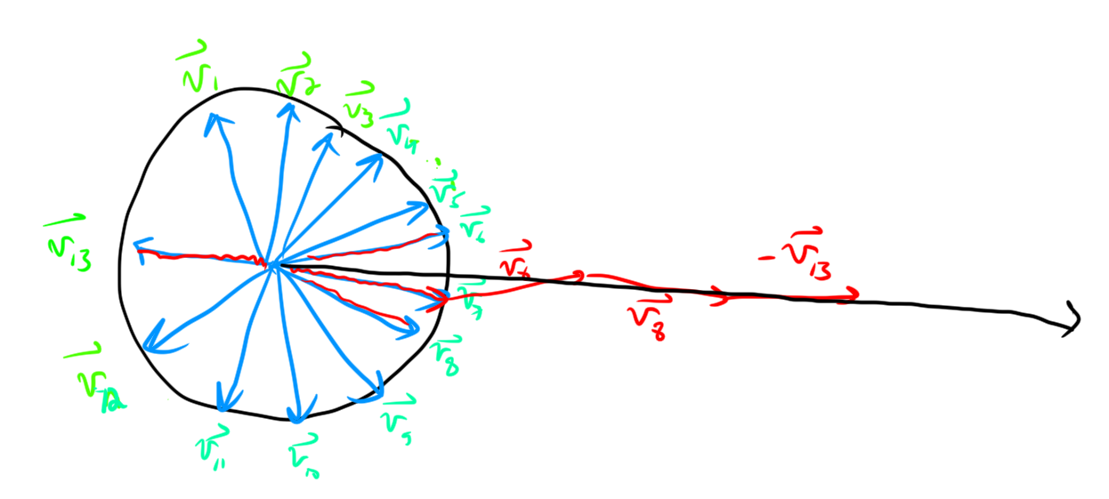
Theorem. Let \(v_1,\ldots, v_n \in \mathbb{R}^m\) be arbitrary unit vectors. Then there exists \(\epsilon_1,\ldots, \epsilon_n \in \{-1,1\}\) such that \[\left| \sum_{i=1}^n \epsilon_i v_i \right| \le \sqrt{n}\] and there exists \(\epsilon_1,\ldots, \epsilon_n \in \{-1,+1\}\) such that \[\left| \sum_{i=1}^n \epsilon_i v_i \right| \ge \sqrt{n}\]
Proof. Choose the \(\epsilon_i\) randomly with \(\Pr[\epsilon_i=-1] = \Pr[\epsilon_i = +1] = 1/2\) (and indpendently). Let \[X = \left|\sum_{i=1}^n \epsilon_i v_i\right|^2 \] Note
\[X = \sum_{i,j} \epsilon_i\epsilon_j v_i\cdot v_j \]
Let’s compute \(\mathop{\mathrm{\mathbb{E}}}[X]\):
\[\mathop{\mathrm{\mathbb{E}}}[X] = \sum_{i,j} \mathop{\mathrm{\mathbb{E}}}[\epsilon_i\epsilon_j] v_i\cdot v_j \]
If \(i=j\) then \(\mathop{\mathrm{\mathbb{E}}}[\epsilon_i^2] = \mathop{\mathrm{\mathbb{E}}}[1] = 1.\) Else, \(\epsilon_i, \epsilon_j\) are independent, so \(\mathop{\mathrm{\mathbb{E}}}[\epsilon_i \epsilon_j] = \mathop{\mathrm{\mathbb{E}}}[\epsilon_i] \mathop{\mathrm{\mathbb{E}}}[\epsilon_j] = 0\)
Overall we have \[\mathop{\mathrm{\mathbb{E}}}[X] = \sum_{i} v_i\cdot v_i = n \]
There must be choice of \(\epsilon_i\) so that \(X\ge \mathop{\mathrm{\mathbb{E}}}[X]\) and so that \(X \le \mathop{\mathrm{\mathbb{E}}}[X]\).
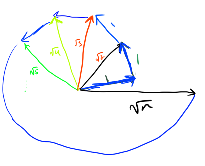
Remark. Furthermore, if you choose the \(\epsilon_i\) greedily, it works.
Let’s say that we are trying to get the resulting vector \(\sum_i \epsilon_i v_i\) to be far from the origin. Greedily choosing them means you flip the vector so that it points in roughly the same directino as the partial sum so far. i.e. make the dot-product \[\epsilon_s v_s \cdot \left( \sum_{i=1}^{s-1} \epsilon_i v_i \right) \ge 0.\]
In the worst case for the vector sum being big this dot product is always \(0\). Then we are kind of spiralling around the origin rather than exploding out. But regardless, even in this trash case we’re good! Here’s a picture showing that greed is good and that even in the trash case we’re rolling.
I’ll try the exercises and put any cool ones I solve here (also for week 1).
Chapter 3
[coming no later than Friday May 22]]
dang it!!! I’m so sorry @my_dedicated_fanbase. I totally forgot about this and stuff. In my defense I was at a hackathon stayed up till 4:30am, and I’ve also been binge-rereading Mistborn (3 700+ page books in 3 days? oops). Agh this blog is falling apart! I’ve done like one of the homework problems so far. aggghhhhh. OK, I’m gonna do better in the future. Anyways, I’m gonna read a bit and go to bed, but tomorrow I really legitamitely will be trying the homework problems and doing some reading. cya!
Update number 2: again, I didn’t get to doing this. I’ve done a bit more of the homework now, but it’s really intense. Honestly I might go and read a different book… I do really want to read that generatingfunctionology book, and I think I can do more of the exercises. I’ll keep trying on the probabilistic method though. I’m not having trouble understanding the proofs, it’s creating them that’s the problem. lol. Anyways, hopefully I can get chapter 3 out soon.
update number 3: ok this section is really coming soon. for real now! I convinced a couple of people to join a little club to read this book with me which’ll be super helpful in terms of reminding me to read :). And just super fun in general.
OK let’s go.
Here’s the big idea for this week:
Random structures are pretty good
But often it turns out that by altering a random structure
you can get somehting even better than what you started with!
This is called an alteration
This is maybe best described by example:
Theorem. Consider the ramsay number \(R(k,k)\). For any integer \(n\), \[R(k, k) > n - \binom{n}{k}2^{1-\binom{k}{2}}.\]
This turns out to be better than the method I originally talked about way back in Chapter 1! In particular we get
Corollary. \[R(k,k) > \frac{1}{e}(1+o(1))k2^{k/2}\]
Corollary. \[R(k,k) > \frac{1}{e\sqrt{2}}(1+o(1))k2^{k/2}\]
Remark. I actually just showed \(R(k,k)>2^{k/2}\), but if I cared more about the exact asymptotics apparenly that’s what the asymptotics come out to.
Remark. Actuall asymptotics aren’t important at all, it’s the method that’s important.
Proof. Randomly color a graph on \(n\) vertices. Let \(X\) be the random variable “number of monochromatic \(K_k\) subgraphs”. By linearity of expeectation \[\mathop{\mathrm{\mathbb{E}}}[X] = \binom{n}{k} 2^{1-\binom{k}{2}}.\] Of course there is some coloring where \(X \le \mathop{\mathrm{\mathbb{E}}}[X]\). Pick such a coloring, and remove a vertex from every monochromatic \(K_k\). Of course this new graph has now monochromatic \(K_k\), we just destroyed them all! But the new graph has at least \[n-\binom{n}{k} 2^{1-\binom{k}{2}}\] vertices, hence the desired claim.