Throughout the post I will generally omit log factors. In some places I have written \(n^{\omega+o(1)}\), but really this should probably be written in most places.
lecture 1
Lots of matrix problems, e.g., matrix inversion, are equivalent to MM or at least closely related to MM.
lecture 2
4-russians: shave some logs by lookup tables of size \(\log n\)
triangle detection to triangle finding
Randomly split vertices in half. Run detection on both halves. Have to try \(O(1)\) times in expectation. The run time would be, in expectation, \[\sum T(n/2^{i})\le T(n) 2\sum (1-\varepsilon)^{i}\le T(n)2\varepsilon^{-1}.\]
This can be de-randomized as follows: split the set into \(6\) equal sized parts. There must be some set of \(3\) of them that contains a triangle. Every set of \(3\) of them has size \(n/2.\)
using triangle detection to do BMM
BMM is defined as \[(AB)[i,j] = \bigvee_k (A[i,k]\land B[k,j]).\]
Remark. You can do BMM via fast MM techniques in \(n^{\omega}\) time.
Theorem. You can also do BMM via triangle-detection. This is asymptotically slower, but kind of nicer because it doesn’t rely on crazy impractical tensor-decomposition stuff with ridiculous constant factors. More precisely, if there is a \(D(n)\) time algorithm for triangle detection then there is an \(n^{2}D(n^{1/3})\) time algorithm for BMM. Using BMM to do triangle detection is trivial. Thus, BMM and triangle detection are “sub-cubic equivalent”.
Proof. Make a tri-partite graph \(X,Y,Z\). Put all the edges between \(X,Z\). Put edges between \(i\in X,j\in Y\) if \(A[i,j]=1\) and edges between \(j\in Y, k\in Z\) if \(B[j,k]=1\).
Split each of \(X,Y,Z\) into parts of size \(t\). For each tripple of little parts eat all the triangles in it.
Run time: \[t^3 D(n/t) + n^{2} D(n/t).\] Set \(t=n^{2/3}\).
more notes
Theorem. transitive closure is sub-cubicly equivalent to BMM
Proof. One direction is like this:
Other direction is like this: compute SCC, topo-sort the SCC DAG Trans-closure of DAG can be done with MM. In the trans-closure, \(A+I\) is upper-triangular.
Theorem. You can compute strongly connected components in \(n^{2}\) time.
lecture 3- intro to APSP
APSP: Given a weighted (possibly directed) graph, compute \(d(u,v)\) for all vertices \(u,v\).
Best algorithm as of 2021 (Ryan Williams): \(n^{3} / 2^{\Omega(\sqrt{\log n})}\).
Observation: \(d(u,v)\) is the smallest \(k\) for which \(A^{k}[u,v]\neq 0\). This is great if the graph has small diameter. For far away vertices we need another technique
hitting set algorithm
Lemma. Hitting sets: Let \(S\) be a collection of \(m\) sets of size \(\ge k\) over \(V=[n]\). Then with high probability in \(m\), a uniformly random subset \(T\subset V\) of size \(\Omega((n/k) \log m)\) intersects all sets in \(S\) non-trivially.
Theorem. There is an \(n^{(3+\omega)/2 + o(1)}\) time algorithm for APSP. even in directed graphs.
Proof. Take a random set \(S\) of size \((n/k)\log m\). It hits all paths of length at least \(k\) by the above lemmma.
Run BFS into and out of each vertex \(t\in S\) so that we get \(d(u,t), d(t,u)\) for all \(u\) in the graph. Then compute \(d(u,v)\) for \(u,v\) which are distance at least \(k\) appart as \(\min_{t\in S} d(u,t)+d(t,v)\).
Balance this against the \(kn^{\omega}\) algorithm for determining \(d(u,v)\) in the case that \(u,v\) are at most distance \(k\) appart.
Siedel’s APSP Algorithm
Theorem. \(n^{\omega + o(1)}\) algo for APSP in undirected unweighted graphs
Proof. Idea:
- If \(u,v\) are distance \(d\) in \(A\), then they are distance \(\left\lceil d/2 \right\rceil\) in \(A^{2}\lor A\).
- if we also had an algo for “parity of distance between \(u,v\)” then we would have a simple recursive algorithm for APSP
- observe that if \(k\in N(j)\) then \(|d(i,k) - d(i,j)| \le 1\). So \(d(i,k)=d(i,j) \iff d(i,k)\equiv d(i,j)\mod 2\).
so it turns out that there is some MM stuff that you can do by looking at the neighborhood of a vertex to determine the parity of the distance, based on the above observation.
lecture 4- Zwick’s APSP Algorithm
Lemma. Dijstra’s algorithm: Given a graph \(G\) with non-negative edge weights, there is an algorithm wtih running time \(O(m+n\log n)\) to compute SSSP.
Proof. (ok but that’s a little bit overly fancy using Fibonacci heaps, reallly)
The algorithm is as follows:
- maintain a min-heap of the vertices based on tentative distance estimates
- Repeatedly take the closest vertex from the heap, and update the distance to all vertices through this vertex
lecture 5- weighted APSP
Theorem. You can also do APSP in weighted undirected graphs pretty fast.
Proof. We again break into cases for short and long paths. We again sample a large set and compute distances from everything to and from all vertices of this set. Now because stuff is weighted this is a bit more complicated, we can’t just BFS.
You do SSSP, Johnson’s trick (i.e., adding the results of SSSP from an auxiliary vertex to the weights to get positive weights), and finally Dijkstra’s algorithm.
For short paths we need a new type of MM: \((\min, +)\)-product.
Remark.
\((A\star B) [i,j] = \min_k (A[i,k]+B[k,j])\)
\((\min, +)\)-product is actually equivalent to APSP. No “combinatorial algorithm” nonsense.
However, it turns out you can compute \(A\star B\) using fast MM if the entries are all small integers.
lecture 6- TODO
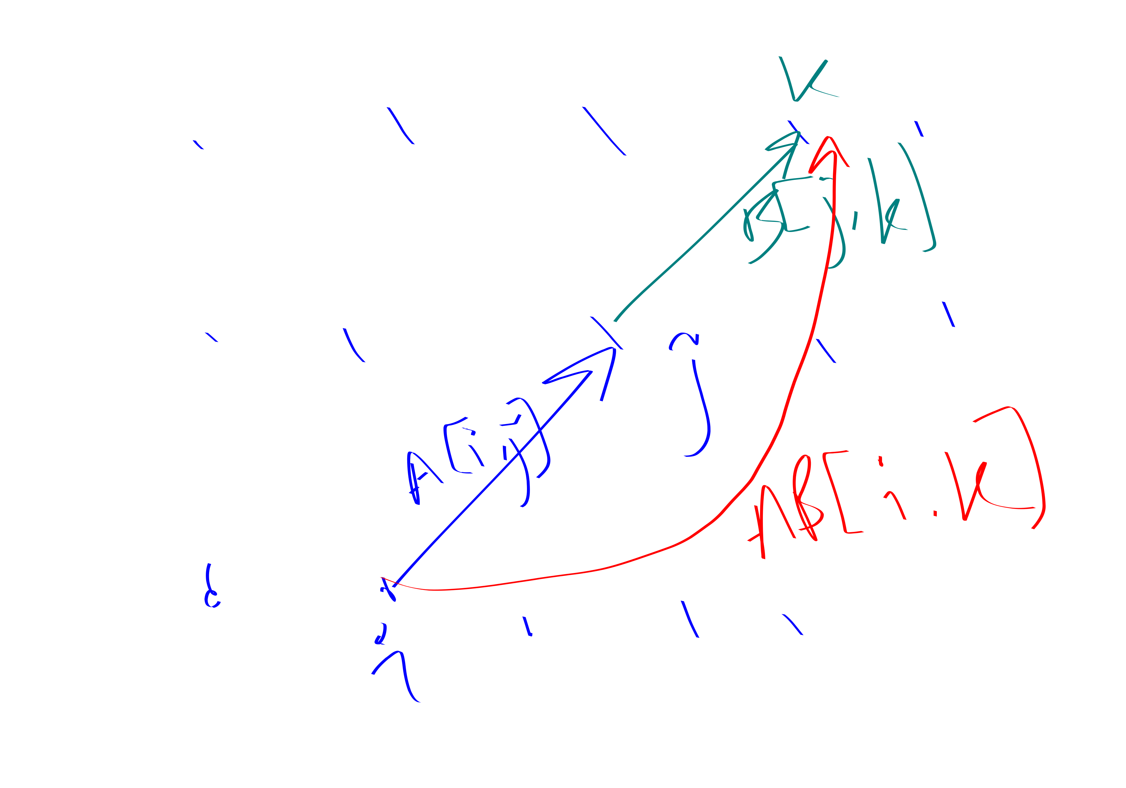
All pairs earliest arrivals, bottleneck paths and the dominance product
All pairs earliest arrivals
Setup is as follows: 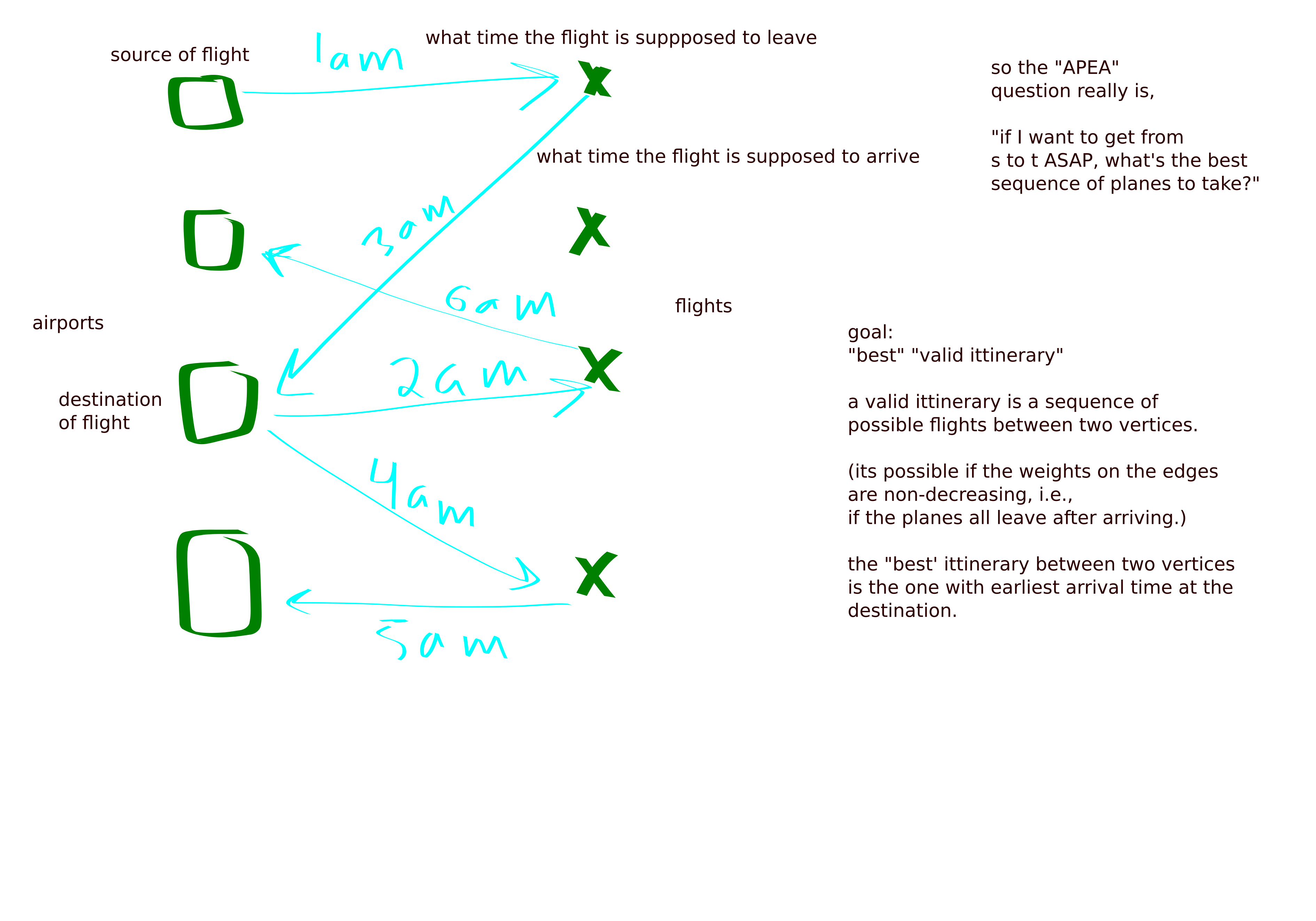
- Flights: source, destination, departure and arrival times
- Airports
- goal: find the fastest route between each pair of vertices
- a route is valid if you could make all the planes
First we focus on the 2-hop version which can be solved via the \(\min, \le\) matrix product.
All pairs bottleneck Paths
Bottleneck of a path: minimum weight edge on the path. For all \(u,v\), find the maximum over all \(u\to v\) paths of the bottleneck weight of the path. For example, if the weight is size of truck that can fit through tunnel we want to find the largest truck that can get between two given points.
max-min product: \[\max_k \min (A[i,k], B[k,j])\]
For more details see my blog post about MM.
lecture 7- Successor and witness matrices; computing actual paths: TODO
lecture 8- minimum weight triangle
Theorem. Minimum vertex weight triangle: vertices are given integer weights. Find the triangle of minimum weight. Can be done in \(O(n^{\omega+o(1)})\).
Proof.
First they give a simple algorithm with sub-optimal running time based on the min-witness product: \[\min \left\{ k: A[i,k] = B[k,j] = 1\right\}.\] Can be computed in \(n^{2.529}\) time using rectangular MM.
some fancier algorithm does better.
Seems like some common themes include duplicating vertex set three times, partitioning into vertex subsets arbitrarily and doing stuff on those.
Theorem. Min edge-weight triangle is sub-cubically equivalent to APSP.
Definition. graph radius: \[\min_v \max_u d(u,v)\] May also want to find such a minimizing \(v\) called a center.
Theorem. graph radius subcubically equivalent to APSP.
Proof. You can trivially compute the diameter by first computing APSP.
the other direction is more involved.
big open question: is diameter subcubicaly equiv to APSP?
lecture 9: subgraph isomorphism (SI)
We have a pattern graph with \(k\le O(1)\) vertices.
- induced
- non-induced
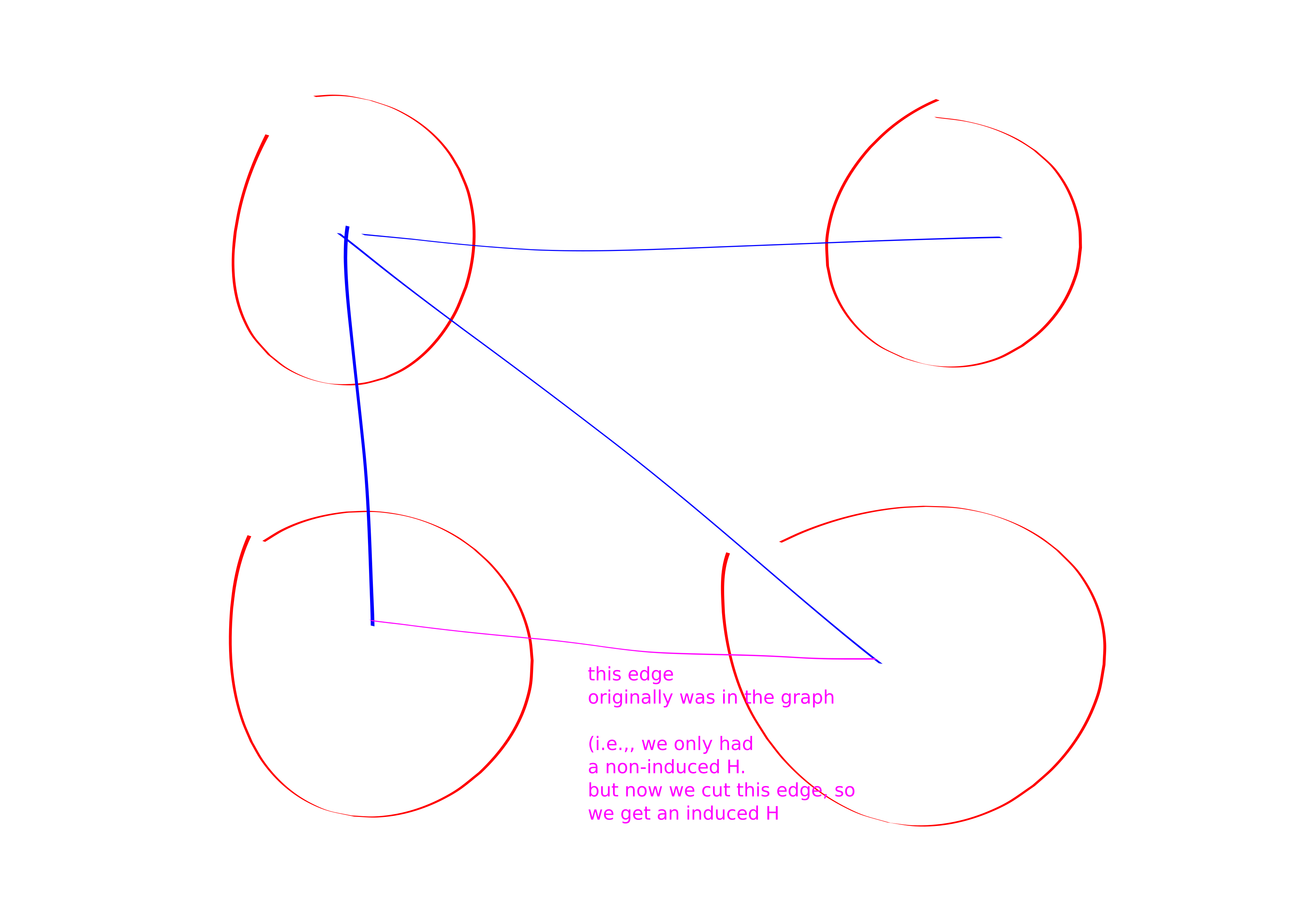
Theorem. We reduce non-induced SI to induced SI.
Proof. Color coding!! Let \(V(H) = h_1,h_2,\ldots, h_k\). Color vertices of graph with \(k\) colors. Let \(w_1,w_2,\ldots, w_k\) be vertices forming a (not-necessarily induced) \(H\) in \(G\). We will hope that \(\chi(w_i) = i\).
After doing the coloring we cut edges between \(u,v\) if \(h_{\chi(u)}, h_{\chi(v)}\notin E(H)\). This turns our non-induced \(H\) into an induced \(H\). The coloring succeeds with constant Pr. Can be derandomized.
Theorem. For any \(k\)-vertex graph \(H\), induced \(H\) reduces to induced \(K_{k}\).
Proof. Color code to make a \(k\)-partite graph. Delete edges internal to the parts. Flip (i.e., if they are present delete them and if they are no present add them) edges \(u,v\) if \(h_{\chi(u)}, h_{\chi(v)}\notin E(H)\).
Now we are looking for a \(k\)-clique.
Theorem. Best \(k\)-clique algorithm [Nestetnice, Poljak. ’85] Let \(k\equiv 0 \mod 3\). Then you can solve \(k\)-clique in \(n^{k\omega/3}\) time.
Proof. We construct a graph on \(\frac{k}{3}\)-tuples of vertices. We create a super-node for a \(\frac{k}{3}\)-tuple iff it is a \(\frac{k}{3}\)-clique. We connect two super-nodes if all edges are present between them. A triangle of super-nodes is a \(k\)-clique in the original graph. Finally, do triangle detection on the super-graph with MM.
But some \(H\) are faster than \(k\)-clique.
\(k=3\)
Theorem. Triangle can be done in \(n^{\omega}\) time: \(tr(A^{3})=0?\)
Theorem. Induced \(V\) (i.e., a triangle minus the third edge) can be found in \(O(m+n)\).
Proof.
- for \(v\in V(G)\):
- do two-step BFS out of \(v\).
- Case 1: the two-step BFS shows that \(N(v)\) is a clique, and is not connected to anything in \(V(G) \setminus (N(v)\sqcup \left\{ v\right\})\).
- in this case we remove \(\left\{ v\right\}\sqcup N(v)\) from the graph and keep going.
- Case 2: if case 1 didn’t happen then we just win.
Each time we do case 1 we spend time \(O(|N(v)|^{2})\) and delete \(\Omega(|N(v)|^{2})\) edges. But we never delete an edge twice. So the aggregate cost of all case 1’s is at most \(m\).
This algo works because in the case 1 case the isolated clique is not ever helpful for finding an induced V, so its super find to just delete it.
\(k=4\)
“Finding Four-Node Subgraphs in Triangle Time” -Williams
- Remark: you can also do stuff based on \(m\) (i.e. sparse graphs)
- diamond approach:
- solve an even harder problem (counting!)
- Let \(A^{2}[i,j]\) denote the number of length-\(2\) paths from \(i\) to \(j\).
- \(\sum_{i,j\in E} \binom{A^{2}[i,j]}{2} = 6\cdot \#(K_4) + \#(K_4-e)\)
- somehow we will restrict to a random subset so that diamond count is not a multiple of \(6\).
- key lemma: Shwarz-Zippel polynomial identity testing: non-zero degree-\(d\) multilinear polynomial has Pr at most \(\frac{1}{2^{d}}\) of being \(0\) on a random point.
- corollary: if you randomly delete half the vertices then with probability \(2^{-|H|}\) the number of \(H\)’s in your graph is not \(0\mod q\) for some prime \(q\), assuming that your graph had a non-zero number of \(H\)’s to begin with.
- then they do sparse graphs!
- and some de-randomization
- The best thing people know for \(K_4\) is \(n^{\omega(1,2,1)}\le n^{3.1}\) (i.e., multiplying \(n \times n^{2}\) and \(n^{2} \times n\) matrices)
“there is a combinatorial algo for \(H\)-detection where \(H\neq K_k\) is a \(k\)-vertex pattern with run-time \(n^{k-1}\).”
CONJECTURE: For any \(k\)-vertex pattern \(H\neq K_k\), \(H\)-detection can be done in \(K_{k-1}\)-detection time.
lecture 12
diameter: largest distance in a graph
why it would be hard to show that diameter is sub-cubically equivalent to APSP (if its even true)
Theorem. There is a simple \(O(n^{2})\) non-deterministic algorithm for diameter.
Proof.
To prove that the diameter is at least \(D\) the PROOF is \(u,v\) with \(d(u,v) \ge D\). To check the proof we run Dijkstra’s algorithm (SSSP).
To prove that the diameter is at most \(D\) the PROOF is a “shortest path tree” out of every vertex \(v\). To check the proof we make sure that the edges in the tree are legit (i.e., actually correspond to edges in the original graph) and then we also check that the distances are sufficiently small.
Theorem. There is a not-so-simple \(O(n^{(3+\omega)/2})\) time non-deterministic algorithm for “zero-triangle” (the problem: does my graph have a triangle with edges summing to \(0\)).
Let \(G\) be a graph with integer weights of absolute value at-most \(n^{c}\) for some constant \(c\).
Proof.
For any prime \(p\) we can count the number of triangles in \(G\) whose weight is \(\equiv 0 \mod p\) in time \(\widetilde{O}(pn^{\omega})\):
This is by using generating functions and cubing the matrix. Specifically, in \(A[i,j]\) we write the polynomial \(x^{w(i,j) \mod p}\). After cubing, the number of zero-sum (mod \(p\)) triangles involving vertex \(i\) is the sum of the coefficients on the \(x^{0},x^{p},x^{2p}\) terms in \(A^{3}[i,i]\).
There is some small prime \(p^{*}\) relative to which there are not so many zero-sum-mod-\(p^{*}\) triangles.
Now, the proof is this prime and a list of all the triangles with zero-sum-mod-\(p^{*}\).
A verifier checks to make sure that all the given triangles are indeed zero-sum-mod-\(p^{*}\) but not actually zero-sum and that all the zero-sum-mod-\(p^{*}\) things are accounted for, in which case there cannot be any real zero-sum triangles.
Proposition. Exact diameter: run APSP.
Theorem. Let \(G\) be a graph with diameter \(3d\) (for simplicity). Then we can give a \(n^{2}+m\sqrt{n}\) time \(1.5\)-approx to diameter.
Proof.
- Let \(T_v\) be the \(\sqrt{n}\) closest vertices to \(v\) for each \(v\).
- Let \(S\) be a size \(\sqrt{n}\log n\)-sized set that intersects each \(T_v\).
- BFS out of all vertices \(s\in S\). Let \(D_1\) be the largest distance found from all these BFS runs.
- Let \(w\) be the vertex that is the farthest from \(S\), i.e., the vertex maximizing \(\min_{s\in S} d(s, w)\).
- BFS out of \(w\). BFS into each \(v\in T_w\).
- Let \(D_2\) be the largest distance found in previous step.
- Output \(1.5\cdot \max(D_1, D_2)\).
correctness: TODO 2.1
performance: TODO 2.2