algorithm class notes

These are some notes on fine grained complexity theory, from Ryan + Virginia’s class. I am not actually taking the class, but am reading the notes. These are now also notes from Ronitt’s Sublinear time algorithms class. I actually am taking this class, but have chosen to digest the material mostly at my own pace. I enjoy having occasional readings about cool algorithms and some occasional problems to work on, and an excuse to think about permutation avoidance again.

I will abbreviate fine grained to FG and sublinear time to SL.

FG lecture 1

Theorem: SETH implies OV

Proof Let be a SAT instance. Break variables into two parts each of size . Make all partial assignments. Then given a partial assignment make a word where you put a at the spot if the partial assignment satisfies that clause, and 1 else. You also have two bits at the front of the vector to indicate whether you are a partial assignment to A or to B. Then, if two vectors are orthogonal, it means that at every spot there is at least one , i.e., one of the assignments satisfies the clause.

Theorem -approximating diameter in is impossible under SETH.

Proof Three part graph. Left: vertex for each vector Right: vertex for each vector Middle: Vertex for each coordinate.

Edges: Connect vector to the coordinates where it has a .

Also add two “star” vertices. Left star vertex has edge to all middle vertices, left vectors and other star Right star vertex has edge to all middle vertices, right vectors and other star.

Then diameter is either 2 or 3. 3 iff orthogonal pair.

lecture 2

Theorem Dominating set in time for .

Proof: = can you get to in 0 or 1 step from ? does meet in the middle. You just need to check if is the zero matrix.

multipoint evaluation We can evaluate a polynomial at points in time. This is FFT.

interpolation Given points you can fit a degree polynomial to them in time.

multiplication You can multiply degree polynomial in time .

3-sum on small magnitude numbers

Theorem Suppose we have a 3-sum instance where the numbers lie in . (you wanna tell if there are 3 summing to zero) We can solve this in time. Let’s go to 3-partite 3-sum with sets . Add to all the numbers and make polynomials. Then you form polynomial . You multiply the polynomials, and check if the coeff of is non-zero.

4-Russians Matrix vector multiplication with pre-processing. Break into blocks. For each block, Store for every . This takes preprocessing time and lets us do evalutaiton in time.

lecture 2 again, but different

ETH: 3-sat requires time for some .

independent set

Example: Encoding a 3SAT instance as an indepset instance.

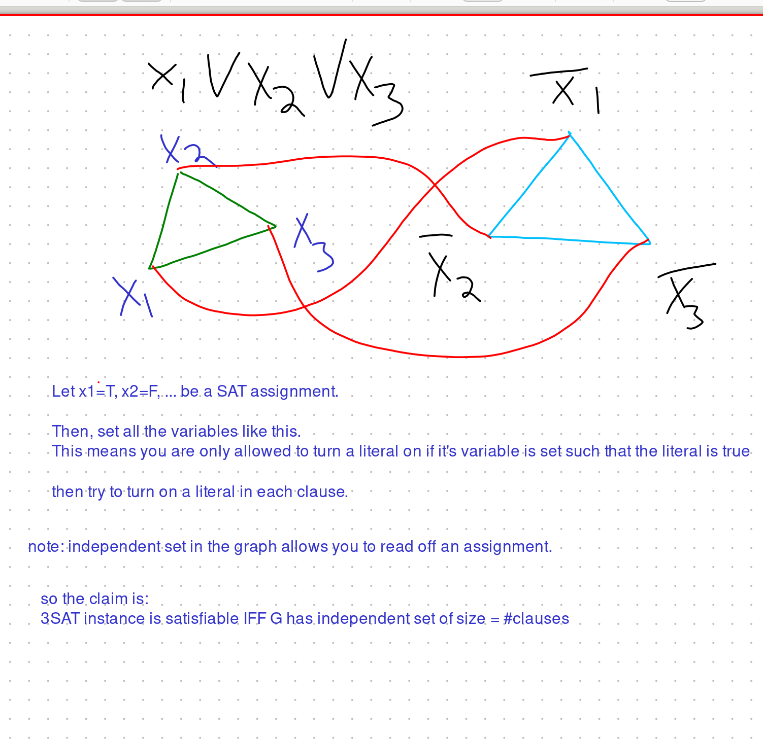
Problem: this doesn’t let us prove an exponential lower bound because we blew up the problem instance too much.

Like you start with a n var m clause 3SAT instance, and produce an m vertex graph. IS algorithm would give you 3SAT algorithm. which is totally possible.

one hope: maybe there is some OP sparsification that we can do.

• probably not.

but, there is this lemma:

IPZ sparsification lemma: there is a time algorithm that takes a -CNF formula on n vars and produces many -CNFs such that F is satisfied iff the or of these is satisfied. Each of these formula guys has n vars and clauses.

yup now the IS thing works.

SETH

For all , exists such that -SAT requires time.

claim: SETH implies ETH even stronger claim: If there is any for which -SAT requires expo time then 3-SAT requires expo time.

Again we use sparsification.

Standard kSAT ⇒ 3SAT reduction: create some auxilliary vars.

Turns a n var m clause kSAT instance into a var clause 3SAT instance.

So first we sparsify. Turn n var m clause ksat into a bunch of n var ~n clause kSAT instances, and then turn these into kn var ~kn clause 3SAT instances.

So if 3SAT were subexponential we would get way too fast of an algorithm for kSAT like this under SETH.

ksum

Theorem: if for all there exists such that -SUM on small numbers takes time then ETH is false.

proof Let’s just work with a sparse formula, by virtue of sparsification lemma. Turns out to be better to work with 1-in-3 SAT (exactly one var in each clause is satisfied to make the clause true). But this only costs us constant blowup to do so its fine.

We do the standard “one-hot encoding” technique. Split the vars into k groups make the numbers:

• have some part of the number to indicate whether you’ve done a partial assignment from each group
• then have some other part for making sure the clauses are all satisfied.

ah this is clever.

Sparsification

OBS: Branching can reduce the number of clauses for example and if you branch on then either you can delete both clauses or you can make them be just 2-variable clauses.

1. consider the variable that appears in the most clauses
2. the fact that we’re not sparse yet means that we can branch and kill some clauses.

SL lec 3

connected components estimation

Algorithm is as follows:

Repeat a couple times:
	pick a random vertex v
	BFS out of v for at most 100/epsilon steps, 
	stop early if you exhaust the connected component.

	define nhat[v] to be either the size of the connected component that v is in, or 100/epsilon if the connected component is big. 

Use the nhat's to guess the number of connected components.

So the key idea behind this estimator is the following observation: If we let be the number of vertices in ‘s connected component and be the number of connected components then we have:

So we are going to compute some numbers with the following property:

Actually, we kind of already talked about how to do this above. Anyways.

So,

And then we need to go into some kind of computation to show that if we have a good approximation on average and we iterate a couple times we can get a good approximation with decent pr. In particular you can just do a Chernoff bound. Specifically, Hoeffding bound says: if are independent random variables taking values in , then the chance that their average deviates from it’s expectation by more than is at most . For us this gives a constant pr of the average successfully being good, which is what we wanted.

MST estimation Kruskal’s algorithm says that to find an MST you can do the following stuff:

• add as many weight edges as is possible.
• then do weight
• etc.

This allows us to relate MST estimation to estimating the size of some connected components defined by taking all edges with weight smaller than some threshold.

todo: add details

SL lec4

Today we are going to talk about a sublinear (in ) time algorithm for coloring a graph.

Sparsification lemma If you sample colors from that each vertex is allowed to use, then probably the graph is colorable using colors from these lists.

proof: We’ll do it below.

Claim: Once we’ve sparsified the color palettes, we can ignore edges where have disjoint palettes. Doing so leaves us with only edges on average (and even whp).

Proof For each vertex , let’s count the number of times a neighbor has a color from ‘s palette; note that if a neighbor shares multiple colors, we get points for each of these. Let be the size of the color palettes. If we fix a neighbor and a color from ‘s palette then has color in it’s palette with probability . Thus, the expected number of times a neighbor shares one of ‘s colors is like . Thus, the expected number of neighbors of is

Now we give a time algorithm for coloring. Note that the trivial greedy algorithm runs in time , so combining both algorithms we can do .

Algorithm

• Sample some random colors for everyone.
• Construct sets which are the set of vertices with color in their palette.
• Construct the sparse edge set as follows:
• For each ,
  • For each pair of vertices
  • Add to if This takes time

Finally, do the greedy algorithm in this sparse graph.

sparsification lemma
We don’t actually prove the sparsification lemma. we prove something a bit weaker: we allow colors. Anyways the proof is as follows:

• run the greedy algorithm
• show that it fails with pr at each step
• union bound

SL Lec 5

In these notes VC will refer to vertex cover (a set of vertices that hits every edge).

Q: How to approximate min VC size in sublinear time? A: We will give a distributed algorithm for computing a small vertex cover.

More precisely, after running the distributed algorithm, every vertex should raise a flag saying whether or not they wish to participate in the VC.

We work in the LOCAL model of distributed computation.

We let denote the max degree of the graph.

Distributed Vertex Cover Algorithm

for each edge e:
	Initialize x[e] = 1/Delta
for i = 1  ... log_{1+gamma}(Delta)	:
	for each v that has sum_{edges e incident to v} x[e] >= 1/(1+gamma):
		add v to the VC
		for all e incident to v:
			freeze e
	for each unfrozen edge e: 
		multiply x[e] by 1+gamma

Claim 1: This algorithm outputs a VC. pf: Endpoints of frozen edges are added to VC. All edges are eventually frozen.

Claim 2: We can interpret the final values of as a fractional matching. This just means that for all . This fractional matching will satisfy:

Proof We only increase edge weights if we’re sure that it’s safe to do so. The fact that our VC size is not much larger than the fractional matching size can be seen as follows:

• Suppose we form a sum by starting at and then adding to whenever we freeze an endpoint of .
• Because we freeze every edge eventually, at the end we will have .
• The amount that we increment by when we freeze edges incident to some vertex is at least by design.
• Thus, .

Claim 3: The value of a fractional matching gives a lower bound on the size of the minimum vertex cover.

pf This is super obvious for matchings. For fractional matchings, assign each edge to an endpoint in the VC. Have each VC vertex aggregate its assigned edges weights. The total weight aggregated by the VC vertices is , and it is at most per vertex. QED.

SL Lec 6

Last class I think we got a approximation to min VC.

CAUTION: maximal maximum

In this lecture we will talk about approximating the size of a maximal matching (?) Let be a maximal matching and let be a minimum Vertex Cover. Observe: .

Claim: a maximal matching has size at least

pf: each edge you take eliminates fewer than edges as options.

Greedy Maximal matching alg:

• take edges until you can’t take any more

Now we have an interesting idea:

• Imagine we had an oracle that would tell us whether an edge was in the matching.
• Would that help?

For estimation it totally would. We would just sample some vertices to estimate the probability that a random vertex is an endpoint of an edge of the matching.

And we add a bit just to guard against terrible underestimates.

ok fine so this’d be great if we had such an oracle.

Intuitively: maybe we don’t need to actually run greedy to figure out it’s bx on an edge?

Here’s a weird (but useful) recursive way of writing out our greedy algorithm

def matched(e):
	for all edges e' adjacent to e that come before e in ordering:
		if matched(e'):
			return False (e not matched)
	return True (e matched)

Let’s try seeing how expensive this is if we do a random ordering.

Under a random ordering, the probability of going on some specific path of length is . The number of paths of length from an edge is at most . Thus, the expected cost of the recursion is:

So we can get a time algorithm for 2-approximate VC (i.e., for computing the size of some maximal matching).

Is this good? Well, I wouldn’t use it unless . But in that case, sure it’s good.

FG 09-27

Virginia showed us a neat trick in class today: breaking the problem up into lots of little parts. Specifically, the problem was dynamic reachability and she wanted to give some combinatorial lower bounds based on triangle detection / BMM. And we could get a simple lower bound pretty easily, but chopping up the problem in a nice way let us get a lower bound even with arbitrary polynomial precomputation.

So that was nice.

SL 7

Property testing for graphs:

• “-far” will mean “can edit ” edges to get in class; here is max degree limit.

Kuratowski theorem planar iff no K5 or K33 minors
minor = graph obtained by contracting edges

Def -hyperfinite if can remove edges to get a graph where all connected components have size .

i.e., Remove few edges to break graph into tiny pieces.

Theorem For all , exists st planar graph of max degree is hyperfinite.

So we can use the following approach for testing planarity:

1. Find a way to remove a small number of edges in order to split G into small CCs.
2. If step (1) fails, we know we aren’t planar.
3. If step (1) succeeds, we can just check one of these little CCs for whether or not it’s planar.

Similar to what we did for matching last time, we’re going to break the problem into two parts: making a “Partition Oracle” and using a Partition Oracle.

Partition Oracle

• input: vertex
• output: Name of the part of the partition that belongs to

Require: partitions are small and connected. Also require: if is planar, then at most edges cross partition.

It’s pretty straightforward how to do testing once you have such an oracle.

Building the oracle

1. global partitioning strategy
2. locally implement it

is a -isolated neighborhood of node if

• is connected \
• edges connecting , are at most

Claim: in a planar graph, in any decent partition most nodes have -isolated neighborhoods. I don’t follow this yet, but let’s keep going.

Global Partitioning algorithm (note: I don’t think we actually do this, this is just how you would in theory glue stuff together?)

order vertices randomly
partition = []
for i in range(n):
	if v_i still in graph:
		if exists (delta,k)-isolated nbrhd of v_i in remaining graph:
			S = this neighborhood
		else:
			S = {v_i} # hopefully this is unlikely
	partition.append(S)
	Remove S from graph

We want to show that this algorithm works reasonably well. Lemma: A -fraction of nodes enjoy isolated nbrhoods.

Proof sketch Using the hyperfiniteness theorem, we know that there is a partition such that if we rm edges, then every CC in the resulting graph has size at most .

For each vertex , let be the number of edges that touch the CC that ends up in once we’ve cut the edges. Then, . In other words,

By Markov,

So basically the global algorithm is pretty good.

Now, this global algorithm is basically just greedy. So I’m hopeful that if we do the same random ordering trick that we did last time, maybe good things will happen. Like we can cut long range dependencies and just locally simulate the greedy thing.

Local Simulation of Partition Oracle Yeah so the way we do it is indeed just like last time. (this is not to diminish the technique --- on the contrary, I think the broad-applicability of this technique is exciting!) But even having seen last time it took me a minute to see this so let me write it down.

Here’s a recursive version of the local oracle:

# fix a random ordering of the vertices
# input: vertex
# output: a small neighborhood of v that has few edges to the outside world
# note: these neighborhood things need to be **consistent** across calls to the oracle
def oracle(v):
	for each vertex w within distance k of v, where w has lower rank than v:
		run oracle(w)
	if some nearby w already claimed v:
		output the part that claimed v
	else:
		just do a little BFS out of v (respecting the nearby guys who have their own thing going on) and decide on a neighborhood for v

Running time analysis is as follows:

for recursion-y stuff. (Also, who thought that doubly exponential running time was a good idea?) (lol I guess think of as constants, then this is pretty good).

Anyways, then we have to do the little BFS thing, but this is just small money in the total running time.

Apparently you can do much better dependence on . ok.

property testing lower bounds

Problem: Given , find a vector such that . Queries that you’re allowed to make: You can choose any vector and ask for .

Claim:

You can’t solve this problem using fewer than queries.

Proof: Suppose that you had some (potentially randomized) algorithm that could output a vector such that in time . Then, we could by symmetry have a randomized algorithm with the property that for each , . Then, if we ran this times and took a majority vote, we would have an estimate that is correct with probability for each coordinate of . Taking a union bound, we have that with probability we have actually just recovered . This is information theoretically impossible to do faster than — we only get one output bit per query. Thus we must have . So .

Remark: I’m pretty sure that you actually need queries, but haven’t thought about how to make the lower bound tighter.

FG — matrices

Solve LCA in assuming . First, compute all of these guys:

Then just do something easy to get

SL SPANERS

Def: -spanner is a subgraph such that

Remark suppose is a -free bipartite graph with about edges — note that such graphs exist. Suppose we remove an edge from . Then, there is no path of length between the vertices that we just deleted an edge between.

This is a proof that edges are required to get a -spanner.

Similar lower bounds for other assuming girth conjecture.

Today, we give an LCA algorithm for computing a -spanner with edges. We will be able to make queries of the form “is this edge in the spanner graph?” in time.

First idea: We can delete an edge from every triangle.

For today: We assume max-degree . ok, fine.

First, how would you even do this globally?

1. Pick random set of size
2. Then, has neighbor to all high degree vertices.
3. Now we construct a graph as follows:
4. Add all edges touching
5. Add all edges touching low degree vertices
6. Add ONE edge from to all adjacent clusters

This graph clearly has a very small number of edges.

Suppose is an edge and both are high degree vertices. If are in the same cluster, then if is the cluster center we have a length path . If are in different clusters, then let be the cluster center of ‘s cluster. We know that is an edge, and that has an edge to some which is in ‘s cluster. Overall, we deduce that is a path that exists.

side remark — I quite enjoy some algorithmic graph theory! brings back some good memories. anyways.

other side remark: in our model of the graph, we allow “degree probe” i.e., asking in constant time what the degree of a vertex is.

Anyways, that was the global algorithm. Now, let me try to guess how I’d local-ify it.

So, in a LCA you have query access to some huge random string that is persistent. Like your algorithm is parameterized by this random string, and just has to work for most choices of this random string.

So ok, each vertex picks whether it’s a center or not. So now it’s pretty easy to pick out the edges touching low degree vertices, and also the edges touching centers. Also, it’s pretty easy for every vertex to choose it’s cluster center that it wants to join — just join the cluster who’s cluster center has the lowest id amongst all clusters that you’re connected to

And then each vertex chooses the lowest id neighbor in each cluster as it’s connection in that cluster. By which I mean, iterate over your neighbors in order, maintain a list of clusters that you’ve already connected to, and take an edge whenever it goes to a new cluster — and ofc at that point you mark that cluster as having been visited. Ah, but this is kind of expensive, because it already takes like ~ time to even find the cluster center of a vertex… so this is probably not quite gonna cut it.

Anyways, let’s think about it. Type 2 query — asking if an edge should exist in virtue of being the lowest id neighbor of which is a center. This should take about time because you just go through neighbors of until find one, but you’re very likely to find one after like tries.

Type 3 query — edge to adjacent cluster??

---

Anyways, that didn’t quite work so we’re changing things up a bit.

Let denote the set of centers that are in the first indices of ‘s neighbor list. Fact: if is high degree, it’ll have between and many such centers.

So, now we’re going to connect to all of . This makes it really easy to check, given a cluster center whether is in ‘s cluster — although this is because we have some kind of weird graph model where I’m allowed to ask for the index of in ‘s adjacency class. It still takes like time to find the cluster centers of a vertex, but checking mmembership is super easy now.

now, here are the other edges that we add:

• For each edge
• Let be the set of neighbors of which are lower id than
• For each , compute and cross off as “we’ve already met”
• If by the end of this process there are some things in that haven’t been crossed off, then we say that the edge is cool and we add it. Else, we don’t add it.

This clearly works, but it’s too slow still

Now finally, here’s the smarter method that’s actually efficient.

Yeah, so we were just being a little bit silly above. Here’s how you can do it fast:

1. For each edge
2. Let be the set of neighbors of with lower id than
3. For each
4. For each
5. Check if is a cluster center of — if so cross out
6. Check whether any didn’t get crossed out.

This takes time .

Maybe later we’ll fix the issue about the max-degree being too large. Oh lol actually we’ll fix it on the homework!

maximal independent set — local computation algorithm

This one had some pretty neat techniques. The main one I liked was, somehow breaking the problem into not-super-overlapping sub-parts.

First, we give a distributed algorithm for the problem.

Each round:
	Every vertex randomly tries to color itself with pr 1/(2 Delta)
	Coloring "goes through" if no neighbors also try to color themselves
	if coloring goes through:
		kill the neighbors

We’re going to run this algorithm for steps. At that point NOT EVERYONE will be handled.
Some ppl will be killed, some will be put in the MIS. But some are still undecided. The number of undecided guys is . It turns out that these guys are “well spread out” , and that this is good.

So our LCA algorithm for MIS is going to work as follows — First run Luby for . Then do BFS to find ‘s live CC. Then brute force find lex first MIS of the live CC.

We will show:

Lemma Size of CC is less than This is actually pretty complicated and cool to show.

Define to measure whether survives all rounds Define to measure whether there is a round where tries to color its self and no neighbors try to. Note that doesn’t necc imply that is in the MIS bc is allowed to “try to color itself” after having already been killed. This was kind of a weird notation choice but whatever.

Then, if are distance at least apart, are independent rvs.

PLAN

• large CC ⇒ many nodes at dist 3 apart
• nodes at dist 3 apart ⇒ unlikely to simultaneously survive

Still a bit complicated.

CC ⇒ just only think about a spanning tree for the CCs.

CLAIM

For live CC , there is a tree of size at least in such that the -dist of each pair of vertices in the tree is at least .

Pf: greedily construct the tree

By a union bound, and the fact that there aren’t too many possible trees on vertices, we get that it’s unlikely that has any sized trees. So the live CCs in should be of size at most .

degeneracy

Nathan and I came up with a nice algorithm for approximating the degeneracy of a graph. Unfortunately the actual pset question was much less cool than this (it was about arboricity). But anyways here’s our ridiculous algorithm.

First, define degeneracy of a graph to be the smallest number such that it’s possible to repeatedly strip vertices of degree from the graph and by doing so end up with the empty graph. Note that this is one nice way of quantifying sparsity of a graph.

Observation 1 You can compute degeneracy in time easily. Just repeatedly strip all the vertices with degree less than . (you can binary search to guess )

Observation 2 Now we argue that subsampling edges doesn’t mess with degeneracy too much. The argument is that, if we look at the vertex stripping order from before, then it’s probably still a valid ordering. When you have lots of neighbors in a set, Chernoff says that this number shrinks predictably. And if not then we don’t even care.