inference

I’m tentatively planning to grind through MIT’s “inference” courses.

Specifically, this is

• algorithms for inference
• inference and information

These cover some things like

• graphical models
• information theory
• inference
• information geometry
• thinking about structure of random variables and independence and stuff
• probably other stuff too

These topics seem

1. pretty intellectually interesting
2. the most relevant stuff to ARC’s research agenda (where I’ll be interning over the summer)

I reserve the right to quit if I find some cool research projects / make up some cool research questions myself. However I don’t anticipate quitting currently.

I’ll record my journey of doing this here. I’ll also tentatively plan to make this into a dialogue because I love JJ+shatar+blobby, but right now I just need to write some stuff down.

Day 0 — Dec 12: Likelihood ratio test: If you have two hypothesis, and want to select one to minimize the probability that you select the wrong one, then you should compute Pr(hypothesis X is true given the data) and choose whichever hypothesis maximizes this chance. This assumes that you have some priors on the chance of the hypothesis being correct, and that under each hypothesis you can compute Pr(data).

Day 1 — Dec 13 Read the first couple Alg for Inf notes. First some definitions, then a neat theorem.

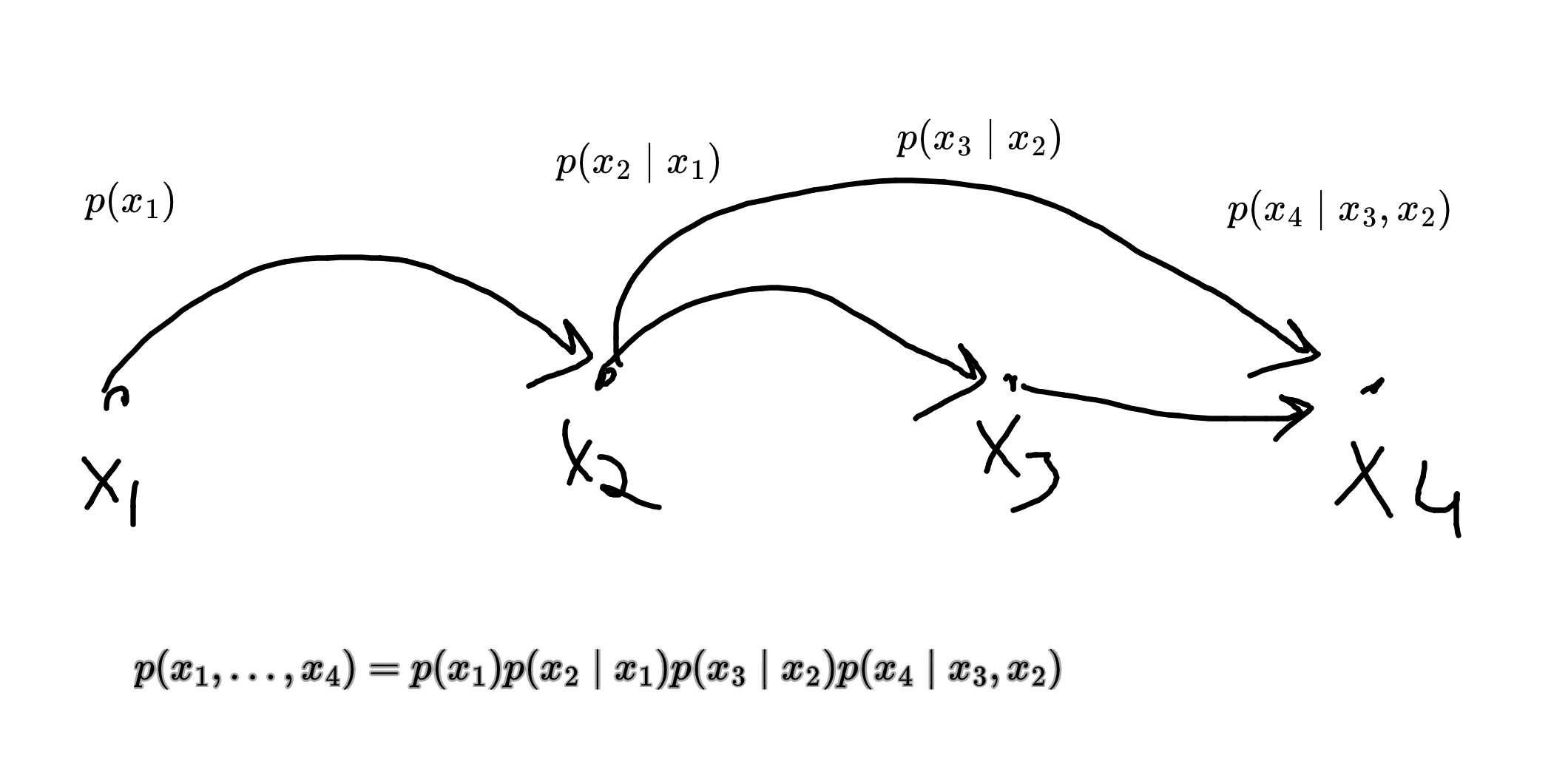
Directed Graphical Model In a directed graphical model, we can factor the probability distribution into terms of the form . So any distribution obeys the conditional independence implied by the complete graph (which is not so impressive since that’s the empty set).

But my digraph implies more independences. For instance, based on my picture.

The general hope for this class is that if we have a sparse graph then we can do much much more efficient things than are possible in the dense case.

A general algorithm for listing off some conditional independences is:

• topo-sort the DAG
• is independent of non-parent things before it in the topo-order, conditional on ‘s parents

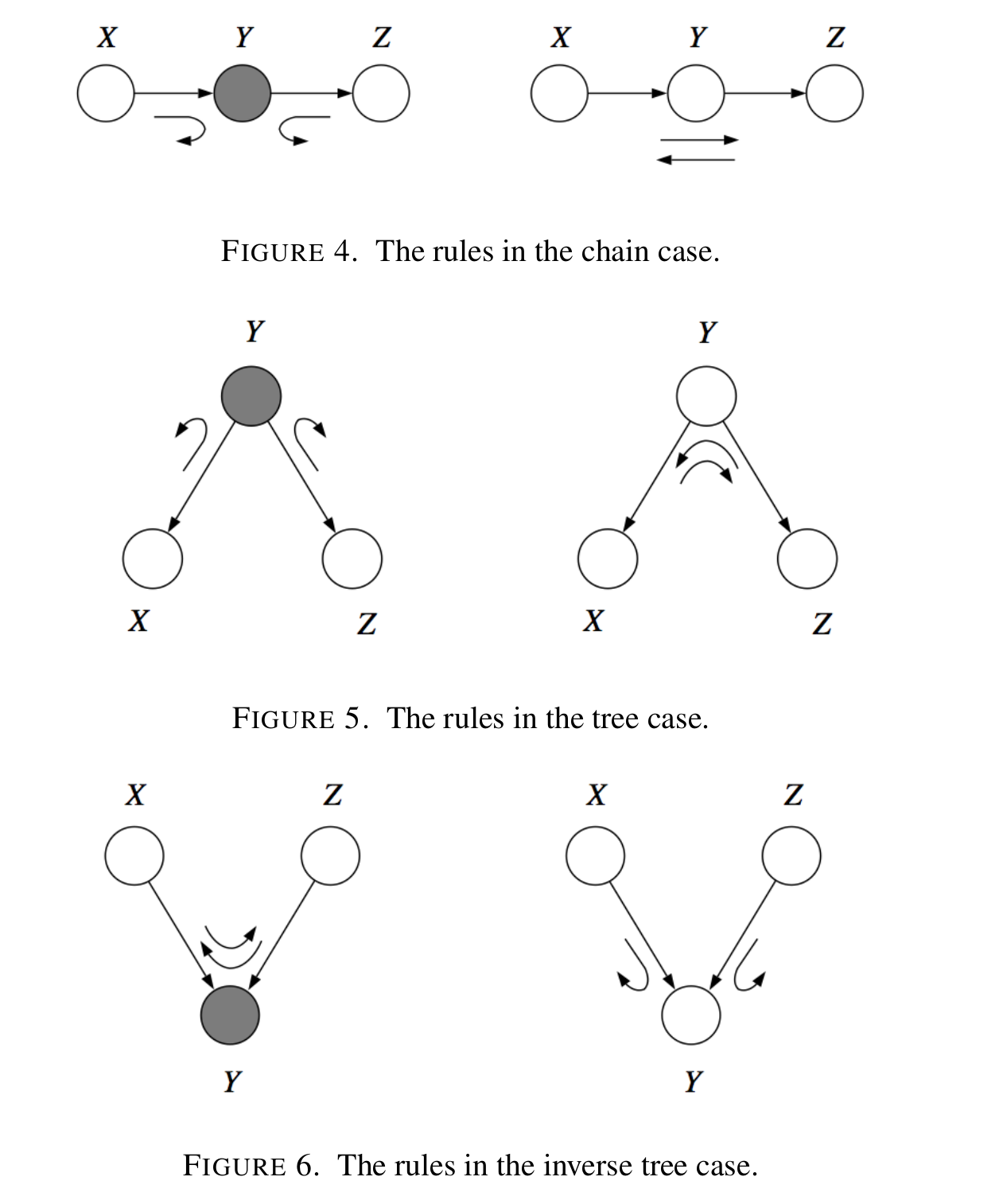
Bayes Ball Algorithm There’s this pretty handy trick for checking whether a conditional independence relation is implied by a directed graphpical model — it’s called the bouncy ball method.

The method answers the question is where can all be sets of variables.

1. Shade the variables .
2. Put a ball at all vertices in .
3. Bounce the balls.
4. If a ball ever hits , then the conditional independence relation is false. Otherwise it is true.

The bouncing is unfortunately a little bit counter-intuitive — it’s not just “when you hit a shaded circle, bounce backwards”. Instead there are three cases:

1. Bounce if shaded on chain. else pass.
2. Bounce if shaded up tree. else pass
3. Pass if shaded in vee. else bounce. The only way I can think of to remember this is to keep these three examples in mind.

Undirected graphical model

Vertices for vars.

Cond. indep

if when you cut , can’t reach from .

This is great and intuitive.

Theorem (Ham-Clifford) (1) If is a pr distr where every state has nonzero pr, and is described by undirected graphical model , then can be expressed as

where is the set of (maximal iyw) cliques in .

(2) If is a pr dist that factors into terms that only look at cliques in , then satisfies the conditional independences specified by cuts ( if cutting separates ).

Proof (2) is a straightforward computation. (1) is quite tricky to prove — I’ll sketch pf below.

We just prove for binary random vars. Probably could generalize. If rvs are binary, say , we can identify with . We’ll conflate and where is the set of coordinates in with value . Now, define

It turns out this function has some nice properties. For instance,

Now we’re going to show that if is not a clique. This will conclude the proof by (*).

To understand why, let’s just consider a graph on vertices with connnections . In this graph we have . Say we’re trying to compute .

By the magic of conditional indepdence we have:

Hence

AND

So,

So You can do the same thing for the terms without the . Basically we’re just using spatial markov property. Anyways, I thought this was neat.

Factor Graph

• bipartite
• one side corresponds to vars, the other side is ways to combine the vars. If the LHS has the vars , and the RHS has vertices then the pr dist must factor as

where is neighbors.

remark: sometimes the models can’t express all relevant properties of your prdist

e.g., directed models seem to be super lossy about preserving conditional independence relations!

Q: can you convert btwn models? A: sometimes.

Day 2 — Dec 17 Wrote up day 1.

Did some of the psets. Note to self — only do the interesting problems: my goal is to be exposed to the subject and understand the basic ideas. If something seems like a technical not interesting or intuitively useful idea, ignore it.

some hw qs

Q1. Undirected graphical model for sampling an independent set according to ? A: the graph is the graphical model.

Q2. Undirected graphical model for sampling a matching according to ? A: orig graph is . Make new graph on the edges where

Day 3 — Dec 18 Talked more about converting between directed and undirected graphical models. Talked about conditions for perfect conversion. Talked about “minimal I maps” i.e., converting to a different graphical model which doens’t imply any false structure but would if you removed any edges.

main takeaways:

• digraph to undigraph conversion is perfect if moralization (connecting parents) doesn’t add edges.
• undigraph has a perfect digraph model iff is “chordal” i.e., all cycles of len > 3 have a chord.

Lec 6 — Gaussian Graphical Models Gaussian:

• for iid Gaussians
• is Gaussian for all
• PDF = covariance rep
• could also write PDF as information rep

Interesting fact: is linear in for Gaussians.

Talked about how to marginalize and condition wrt covariance rep and information rep.

info matrix gives easy way to make graphical models.

• undirected model: add edge whenever
• directed model: idk

Gauss-Markov Process

where are iid Gaussians.

There’s this thing called the Schur complement. Seems important.

• block matrix inversion
• computing marginals / conditioning

Lec 7 Now that we’ve defined graphical models we’re finally going to start actually doing some inference.

Recall — we care about computing posterior beliefs and MAP estimates. Today we think about these problems for undirected graphical models.

Naive alg for marginalization:

Time: . But if we have a nice factorization then we can break up the sum and it’ll have some repeated parts.

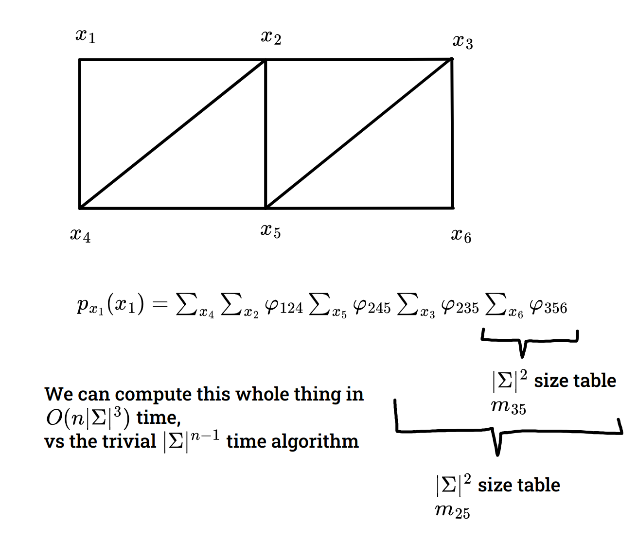
Elimination Alg — will give an exact solution! but may be somewhat computationally expensive. oh this is treewidth — interesting.

Plan going forward I think lectures 8-15 might be good, but mostly look like simple algos like the one above. I think it’d be semi-helpful to know about them, but expect to gain more utility from these other ones

So I’m planning to skip ahead for now to lectures 16,17,18,19 about loopy BP and VI some fancy markov chain stuff, lec 20-24 (end) also seems interesting

could also just try some psets

date xxx: I skimmed all of the notes. Most of the algorithms were not super interesting, they were just pretty obvious DPs.

this is on hiatus for a minute

---

complexity theory

I decided to also learn some complexity theory — i.e., read the Arora Barak book. I’m fairly happy with this decision — it seems like some cool stuff. Here’s what I’ve learned so far.

interactive pfs

Main neat idea here was “how to get rid of the need for private coins”. The basic idea was conveyed to me previously by N (he asked me this question earlier).

Here’s the idea for graph non-isomorphism (GNI): Suppose we have two graphs that we want to test for GNI. Let .

Observe:

• If then .
• If then .

Let . It’s pretty easy to write down a hash function which is approximately pair-wise independent. For instance, for prime works.

okay the approximately thing is kind of annoying. You can solve this by instead choosing to be a power of two, then using hash functions on , and then trimming extra bits somewhere. Whatever, let’s just assume we have a pairwise independent hash function .

It turns out that this gives us a neat guarantee:

Theorem

Let . For any

\rho-\rho^{2}/2 \le \Pr[\exists x\in S \mid h(x)=z] \le \rho.

Proof The upper bound is just a union bound. The lower bound follows by PIE:

Corollary There is a gap of between the probability that exists in the cases and .

proof:

Apparently you can get perfect completeness iyw, I haven’t figured out how yet though.

basic stuff about circuits

decision trees

You can get some pretty strong lower bounds against DTs. Because they’re pretty simple.

One thing that I found pretty interesting was the discussion of vs .

• depth of DT required to compute
• certificate size required to verify

Let’s define a certificate. Fix We say that is an -certificate, if is determined by That is, for all with , .

For instance, if the problem is checking graph connectivity on an -vertex graph, this requires depth DT because for any order (even adaptive) of looking at the edges, it always could be the case that what you’ve seen could be extended to either a connected graph or a non-connected one, until you’ve looked at every last edge.

However, there’s a much shorter certificate that a graph is connected — namely, you could just reveal the edges of a spanning tree. On the other hand, proving that a graph isn’t connected is harder — it requires demonstrating a cut, which could require looking at edges, although this does always suffice.

Anyways the result that I thought was kind of neat is:

Theorem

C(t) \le D(t)\le C(t)^{2}.

Proof The left inequality is obvious.

The right inequality follows bc every positive certificate must intersect every negative certificate, or else a string could have both a positive and a negative certificate!

That is, if we let denote the certificate for then if . And this property is preserved even if we look at some of the bits.

Circuit lower bounds

Hastad’s Switching Lemma Morally speaking this lemma says that for any constants , if you have a -DNF on vars and you randomly restrict of the vars, then with probability something like probably get an -CNF. The lemma is also true if you swap CNF and DNF.

I don’t have intuition for this result yet, but haven’t read the proof.

The switching lemma is used to prove that as follows:

1. Clean the circuit — make it a tree, alternate AND/OR, some other things
2. Repeatedly restrict vars, where is number of remaining vars. This let’s you switch the bottom two layers from AND OR to OR AND (or other way) and then you can do a merge operation which results in the circuit being 1 level less deep.
3. Eventually you end up with a situation where you can satisfy the circuit by just setting a couple variables.
4. This is of course ridiculous because PARITY depends on all the bits.

I got some more intuition for the Hastad Lemma — it’s actually quite likely that a restriction will result in your guy becoming constant . but it’s not likely for whatever you want. although i suspect it is at least like . but anyways the Hastad thing is p useful if you care about this more high probability thing.

There was a neat bound on power of monotone circuits — you need exponentially large ones to compute clique!

I spent quite a bit of time reading the proof that you can’t do PARITY even with MOD3 gates.

The proof has two parts:

1. Anything in ACC0(MOD3) is well approximated by a degree polynomial.
2. PARITY is not well approximated by a degree polynomial.

Proof (1): We go by induction.

• not gates: . no degree increase or approx decay
• MOD3 gates: . degree times 2. no approx decay
• AND/OR: let’s just do AND. if you wanna do it exactly it requires a v large increase in your degree. you can approx it pretty well without boosting degree too much though.

Proof (2): omitted. but I thought it was nice.

Communication complexity Average case hardness Proof complexity